Introduction / Background

Wikipedia a widely used crowdsourced knowledge hub, which presents information in a highly structured format through the use of categories, Wikidata properties and WikiProjects tags[1]. In this project, we aim to analyse the existing categorization, and attempt to automate classification of articles in these categories.

Prior analysis of Wikipedia categories has revealed that it can serve as a reliable source of information[2]. In [3], Mehdi et. al. adopt probabilistic models for topic tagging arbitrary web pages with Wikipedia categories, and in [4], Zareen et. al. develop an ontology from Wikipedia categories to then perform predictions on arbitrary documents.

For our experiments, we extract Wikipedia pages (documents) using MediaWiki APIs with the associated class hierarchy. Each document corresponds to a web page on Wikipedia, and consists of an excerpt its text, and some other useful metadata.

---

Problem Definition / Motivation

Currently, all categorization on Wikipedia is manually performed by individuals in a crowdsourced manner. There are a few issues with this:

1. This may be susceptible to errors and personal biases, despite preventive checks.
2. Manual categorisation is not scalable, for reference, over the last year, around 800,000 new pages were added to Wikipedia each month.

Can we leverage machine learning to better understand how categorisation is currently done in Wikipedia, and build a model to automatically classify articles into topics at scale?

Our goals:

• To examine, statistically, using unsupervised machine learning methods, the effectiveness of the categorization in Wikipedia.
• To classify articles into categories using supervised learning methods capable of learning the information embedded in extracts of Wikipedia pages. As a stretch goal, we aim to test the understanding of the models by classifying questions found in Stack Exchange forums into the forums best suited for them.

---

Dataset Collection and Description

Link to the dataset

We collected our dataset of Wikipedia articles by making use of the MediaWiki APIs. In particular, we made use of the Action API to retrieve Wikipedia page data for 5 major fields:

• Computer Programming
• Fields of Mathematics
• Branches of Biology
• Subfields of Physics
• Subfields of Chemistry

In particular, within each of these categories, we retrieve the subcategories and find all pages belonging to each of these subcategories. In this manner, we retrieve a hierarchical category structure of the Wikipedia pages.

The exact fields retrieved with respect to each web page are:

1. pageid: The unique ID of the page (numerical).
2. title: The title of the page (text).
3. extract: The extract of the page. This usually contains the first paragraph of the page (text).
4. category: The subcategory to which the page belongs (categorical variable).
5. parentCategory: The high-level category to which the page belongs (categorical variable).
6. page_data: The entire raw HTML data of the page (text).

Note that since the page_data attribute contains the entire HTML data. Hence, this data must be cleaned before meaningful analysis can be performed on the text data. The extracts are often used a representative sample of the actual page data for the purposes of analysis of the data.

This resulted in a dataset containing 17,008 samples (articles), spanning a total of 143 subcategories aggregated across all five parent categories. Next, we clean and analyse this dataset, before moving onto machine learning methods.

The files in the link provided above are as follows:

1. enriched_dataset: Directory containing a JSON file for each category with all the fields described above.
2. raw_article_data.csv: CSV of articles across all categories (formed from the JSON files).
3. clean_article_data.csv: CSV of articles across all categories after applying the cleaning steps described below.

---

Data Pre-processing

Data Cleaning

The data obtained in the page_data attribute, as highlighted above is the raw HTML data. In order to preprocess this data to obtain meaningful representations of the pages, we perform the following steps:

1. HTML tag removal: The meaningless HTML tags are removed.
2. Typo correction: Wikipedia pages are prone to having typos. In order to ensure that such typos do not affect our analysis, we make use of an off-the-shelf TextBlob typo correcter.
3. Punctuation removal: Punctuation do not provide any useful context for the purpose of classification, and are hence removed.
4. Diacritic decoding: Diacritics tend to often appear in more scientific when referring to names of scientists which have diacritics. These accents are removed to ensure a consistent word embedding at later stages. Words with such diacrtitics however are not entirely removed, as they can often provide crucial context to determining the category of a page. e.g. Galois -> mathematics, Darwin -> biology.
5. Double space removal: Unnecessary and extraneous spaces are removed from the text.
6. Stopword removal: Stop words are removed by using the standard nltk stopword list. These do not provide useful information towards the purpose of classification.
7. Mathematical notation removal: Since our categories are largely academical, mathematical notations and symbols were present, and latex code was commonly used to represent these. These are not necessary for our analysis, so they were removed.

As a result of this comprehensive cleaning, we end up with a dataset of Wikipedia pages largely containing data which should provide crucial information towards the task of classification. Before we proceed to actually perform classification/clustering however, we first explore our data to understand better its nature.

---

Exploratory Data Analysis

Category Distribution

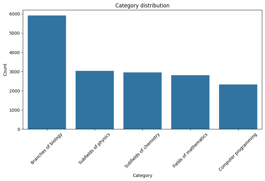
The split of web pages among the 5 parent categories are as follows:

Figure 1: Category Distribution

Key Observation: We observe here that the category “Branches of Biology” dominates the others. We will later work towards accounting for this issue, and also analyze what happens if we choose not to do so.

Subcategory Distribution

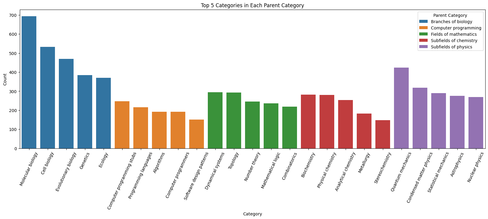
We plot the top 5 most frequency subcategories within each category to determine if a significant dataset imbalance is present within each category itself :

Figure 2: Sub-Category Distribution

Observation: While we can see that as expected from the observation above, the total number of pages from the biology dominates the pages from the other categories, the subcategories within each category are not too badly imbalanced themselves. Hence, it may suffice to simply balance at the granularity of the high-level categories.

Word Count Distribution

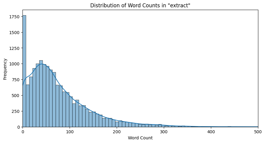
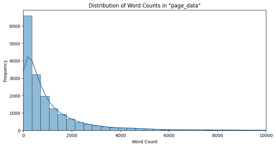
We now plot the word count distribution across the extracts and page data of all the pages:

Figure 3: Word Distribution in Extracts

Figure 4: Word Distribution in Page Data

Observation: We observe here that we have a normal distribution of extract lengths skewed to the left. This is expected because there would be some bias toward shorter length extracts on Wikipedia pages. In the case of page data, the counts seem to be more heavily skewed toward the shorter length pages, but since the bins are very large for the large, as we can see by the kernel density estimator plotted, we still truly do observe a normal distribution which is skewed to the left.

Word Distribution

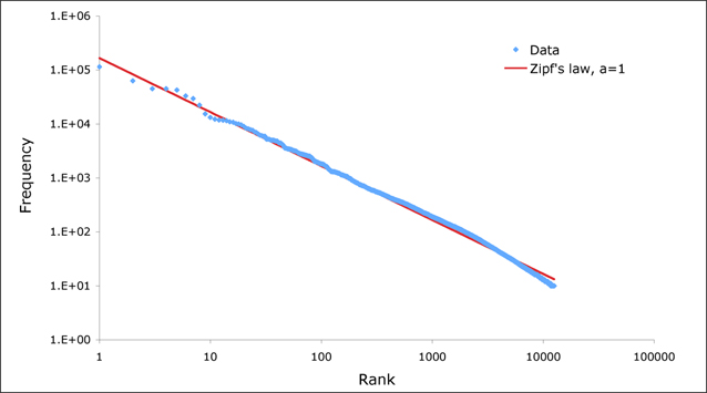
Next, we analyze the word counts. What we expect to see is a distribution that follows Zipf’s law which states that the frequency of the $n^{th}$ is proportional to $\frac{1}{n}$. This is an indicator of a large enough distribution of text data; if a text corpus does not follow Zipf’s law, it is likely that it is not large enough to be representative. The log plot we expect to see is something that looks like the following:

Figure 5: Expected Zipf Distribution (image retrieved from link)

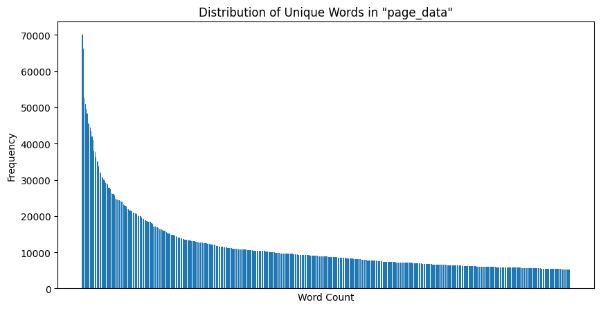
Now, we plot the unique word count distribution for the top 500 most frequent words across all pages retrieved:

Figure 6: Unique Word Count Distribution

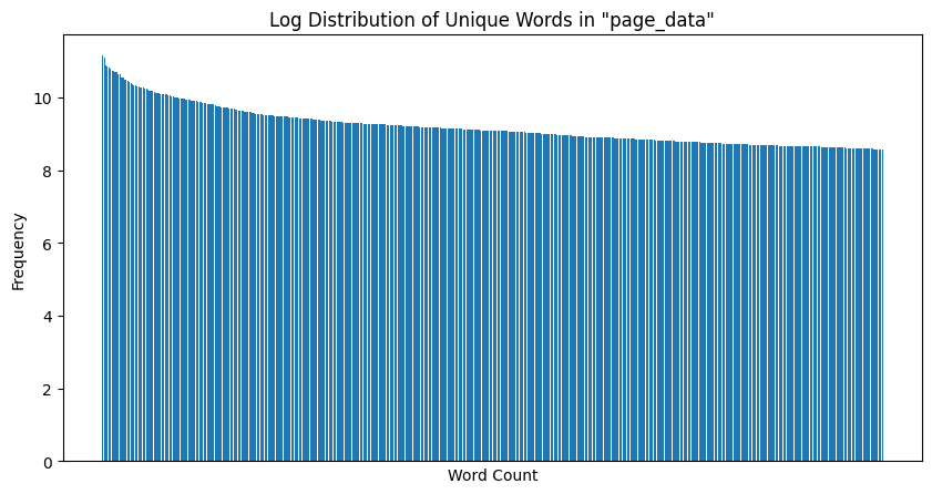
The log plot for the above is as follows:

Figure 7: Unique Word Count Log Distribution

Observation: Here, we see a marked inverse relationship between the $n^th$ most frequency and its corresponding frequency, as evidenced by the roughly liner relationship in the log plot. Hence, Zipf’s law is satisfied quite strongly, and our page data is a good candidate for performing text analysis.

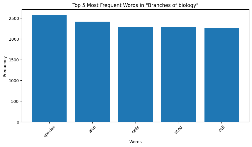
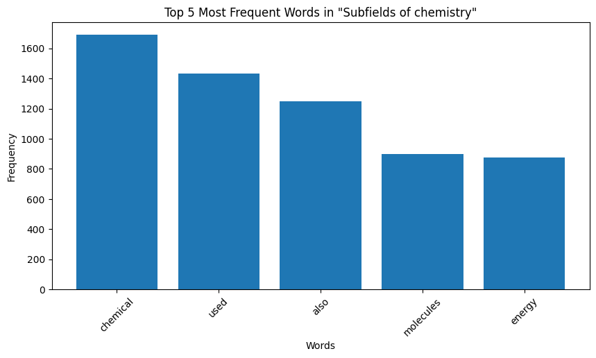
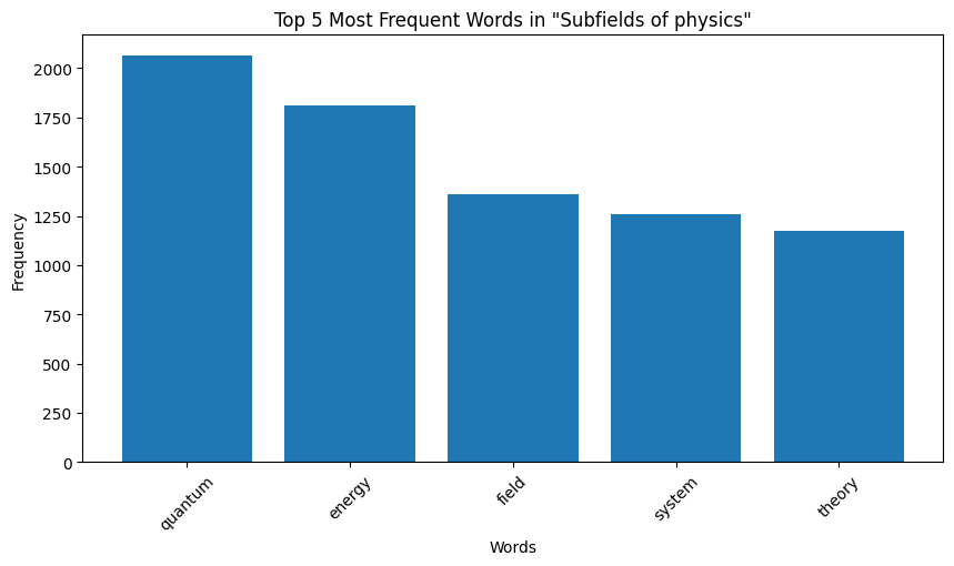
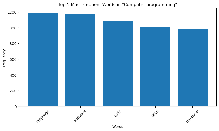
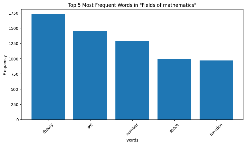
Finally, to get a sense of what words are characteristic of the different categories, we make plots of the word counts per category as follows:

Figure 6: Word Distribution in Extracts for Biology

Figure 7: Word Distribution in Extracts for Chemistry

Figure 8: Word Distribution in Extracts for Physics

Figure 9: Word Distribution in Extracts for Computer Programming

Figure 10: Word Distribution in Extracts for Mathematics

Key Observation: We observe that the top occurring words in the categories are sometimes meaningful, for instance, “species” for biology and “quantum” for physics. However, some meaningless words also appear in the mix. For instance for both the chemistry and biology, “also” is one of the top 5 most frequent words, and “used” occurs very frequently for computer programming. These words are in no way indicative of the true category of the page data. We make a note here of this issue, and delegate the handling of this to the word embeddings we later generate.

Bigram Visualization

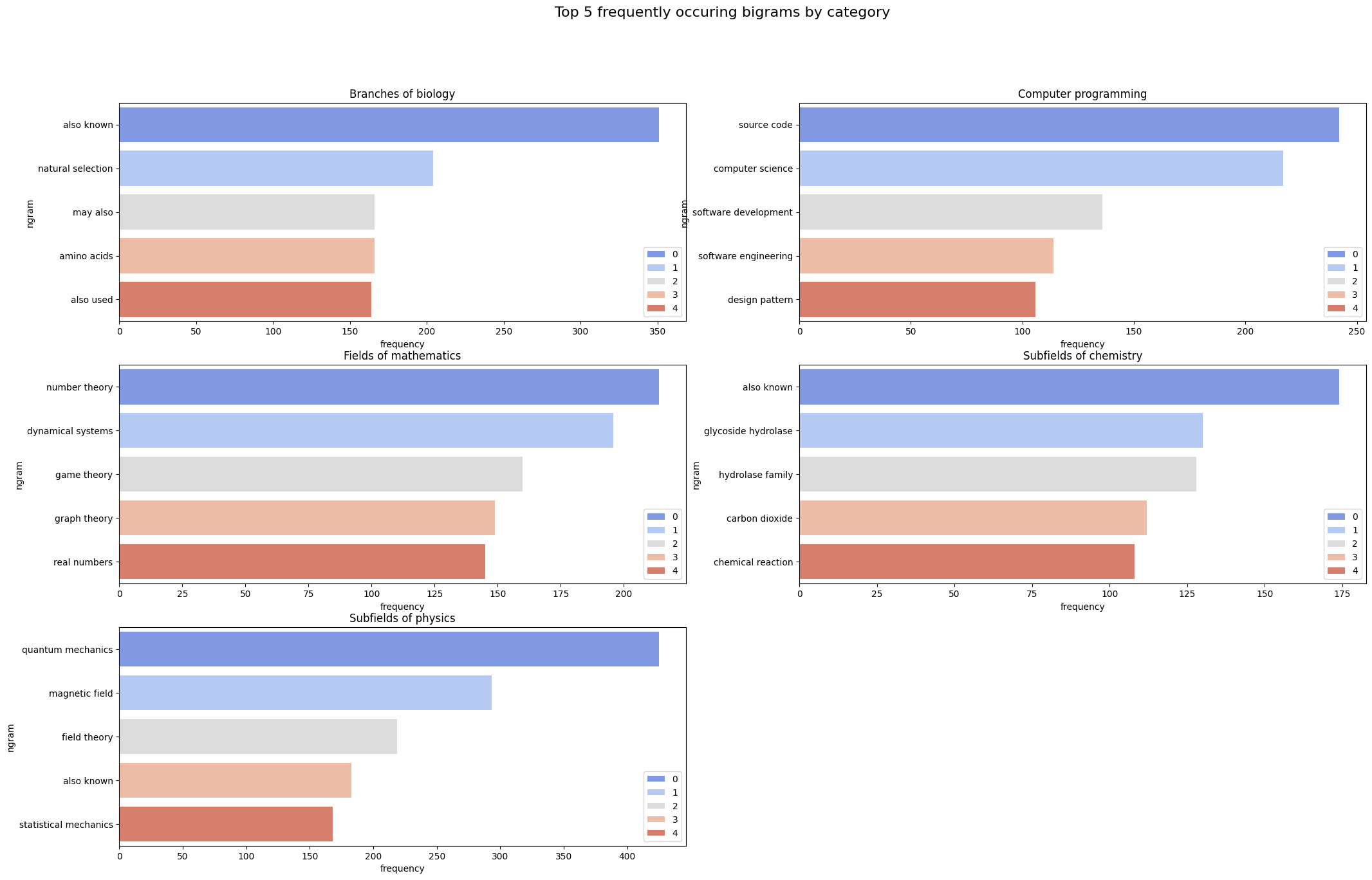
Now, we note the distribution of bigrams in our dataset. This will give some key insights into whether meaningful bigrams occur frequently for the respective categories, and hence whether sequential models like recurrent neural networks (RNNs) and Long Short-Term Memory (LSTM) networks would be effective.

Visualizing $N$-grams for $N > 2$ would in fact give further insights, however we do not do this due to computational limitations. The following is the plot of the most frequent bigram per category:

Figure 11: Bigram Distribution for Different Categories

Observation: Once again, what we observe is that certain meaningful bigrams (like “source code” for computer programming and “dynamical systems” for mathematics) appear, but so do some meaningless ones (such as “may also” for biology and “also known” for physics). Once again, we choose to delegate the handling of this issue to the word embedding generation step.

---

Representation

Since we are dealing with a natural language processing task, one of the key steps in the machine learning pipeline is to develop an efficient representation of the text corpus we have. We denote the set of documents $D$ (Wikipedia page text in our case), and the vocabulary of size $V$ (the overall set of words appearing across all these pages). We need a mathematical (vector) representation of each document. In order to achieve this, we make use of $3$ famous vectorization strategies, which all come built-in with scikit-learn and $1$ co-occurrence based pre-trained word embedding technique:

1. Count Vectorization: This technique of creating word embeddings maps each document $d \in \mathcal{D}$ to a vector in $\mathbb{N}^{V}$, which represents the count of each possible word from the vocabulary in $d$. The rationale of this vectorization scheme is to assign importance to words in the document based on the number of times they occur in the document. Note however that it does not encode any global information about the distribution of words across the entire set of documents.

2. TF-IDF Vectorization: This technique of creating word embeddings maps each document $d \in \mathcal{D}$ to a vector in $\mathbb{N}^{V}$, where the entry in the vector corresponding to a certain word $w \in V$ is computed as its frequency in the document $d$ divided by the number of documents it appears in (known as the document frequency). In practice, often, the log of the document frequency is taken rather than the raw document frequency itself. The rationale of this vectorization scheme is that the most important words are those that occur in only a few documents, but with a very frequency within those documents. For instance, in detecting the category physics, the word “quark” would potentially appear very frequently in documents in the category physics, but appear in only in (relatively) few documents overall.

3. Hashing Vectorization: This technique of creating word embeddings is similar to the Count Vectorization, except that hashing is made use of to obtain a potentially more condensed vector representations. This is largely used to save data. However, a downside of this method is that there is low interpretability since the original words cannot be retrieved, given a certain entry of the vector.

4. GloVe embedding: In this approach we use the pre-trained GloVe embeddings [5] rather than creating our own representation. While the embeddings above rely on the occurrence (or lack thereof) of certain terms, for effective clustering/classification, using context-aware representations might be important. GloVe embeddings are trained in an unsupervised manner, and often try to represented semantically related / co-occurring terms together, even providing some linear relations between the terms in the embedding space.

Recall from our analysis on the word distribution that several highly frequency terms across documents were meaningless. In order to deal with these terms, we set a threshold of 0.25 document frequency when vectorizing using the Count Vectorization and TF-IDF Vectorization strategies; this means that if any word has a document frequency of 25% or higher, it will be considered an insignificant (meaningless) word and be discarded. On generating the embeddings, we obtain representation in the following spaces:

1. Count Vectorization: $\mathbb{R}^{986058}$
2. TF-IDF Vectorization: $\mathbb{R}^{986058}$
3. Hashing Vectorization: $\mathbb{R}^{1048576}$
4. GloVe Vectors (pretrained on Twitter data): $\mathbb{R}^{25}, \mathbb{R}^{50}, \mathbb{R}^{100}, \mathbb{R}^{200}$

These spaces are, unfortunately, still far too large and pose 2 major challenges:

1. There would be a massive computational overhead to using these embeddings directly.
2. They would impose a lot of noise; irrelevant words would cause models to sway away from the true answer due to slight variations in different dimensions.

To simultaneously deal with the above 2 challenges, we make use of (unsupervised) dimensionality reduction techniques. (We omit the dimensionality reduction for GloVe vectors since there are available in 25, 50, 100 and 200 dimensions.)

---

Dimensionality Reduction

We apply one of the most common dimensionality reduction techniques in the context of natural language data:

Latent Semantic Analysis (LSA): Conceptually, this technique simply uses the truncated SVD method of dimensionality reduction. It differs from PCA only in that it does not centre the data. This technicality allows for the operation to be performed efficiently on sparse matrices, which is what we work with in our context, due to extremely large size of the embeddings generated.

We choose to generate embeddings for the dimensions [2, 3, 5, 10, 50, 100] to have a range of potential embeddings to work with and to determine which one is the most representative of our dataset. In the following plots, these embedding sizes are referred to as “number of features”. We do not apply LSA for GloVe as the pre-trained embedding sizes are already in a smaller range.

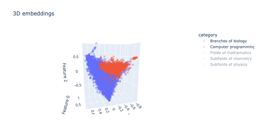
In order to visualize the dimension-reduced embeddings, we make plots of the 2-dimensional and 3-dimensional embeddings (as the rest are not feasible to visualize). Since we know the ground truth category for each document, we plot them by color to observe their separation in the reduced 3D space. The plot below is the visualisation of Count Vectoriser embeddings.

In the above interactive plot, you may click on a certain category to remove those points from the plot. There is overlap between the documents of the 5 categories, which is expected since the embeddings are based on distributional statistics and not semantics. Despite this, there are useful insights we can draw looking at specific categories:

1. The class Biology has a quite distinct boundary compared to the remaining classes, except for chemistry where there is a significant overlap. Biology seems to uniquely cover the Feature 2 interval of [-0.5, -1] and Feature 1 interval of [0, 0.6], which other categories do not.
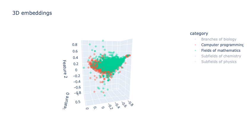
2. The remaining classes often overlap to a great extent. This is expected for pairs of classes like {Mathematics, Physics}, {Mathematics, Computer Programming}, etc. However, for pairs such as {Mathematics, Chemistry}, one would hope that there is a greater distinctions in the points of the classes.
3. Biology and Computer Programming are quite well separated, but Computer Programming and Fields of Mathematics do have overlap, which is expected since their topics are often highly interrelated. The plots below show these cases:

Figure 12: 3D embeddings visualisation after LSA

Figure 13: 3D embeddings visualisation after LSA

Hypothesis: We suspect that the above phenomenon occurs due to the fact that LSA maximizes the variance in the direction of “Biology vs. All” when the number of dimensions is reduced to 3. Our hope is that this issue would be alleviated in higher dimensions such as 5, 10, 50 and 100.

---

Methods

Unsupervised

K-Means

We first make use of K-means to determine the ideal embedding dimension. This is done by training separate K-means models with the optimal setting of K=5, and observing the embedding with the optimal performance, for the Count Vectorizer, TFIDF Vectorizer and Hashing Vectorizer. Upon performing these evaluations, we observe from the result plots obtained that the optimal embedding dimension would be $10$. We state here this result, but more rigorously justify why this is the case based on the result plots.

After this, we analyze whether our $K$-means models are capable of automatically detecting the ideal number of clusters. This is done by making use of the standard elbow plot technique; we plot the inertia against various different values of $K$, and determine the ideal $K^*=5$ that is low enough such that inertia decreases negligibly for higher value of $K$.

Hierarchical Agglomerative Clustering (HAC)

For the more advanced task of classifying at multiple levels, we make use of the sophisticated HAC method. This technique would be very useful in terms of extracting insights about how our data is truly clustered in the latent space. We would hope that, for instance, subfields of mathematics like topology and set theory are closer together in space rather than topology and zoology, a subfield of biology. We perform this method on each of the embedding methods: count, TFIDF and hashing, and for several different reduced dimensions.

Our observations are that this method does not perform very well, but the dendrogram plots obtained give us a good indication on the distribution of the classes in the respective embedding spaces. We investigate in detail the results from this method in the Results section.

Extra: Latent Dirichlet Allocation (Topic Model)

Another unsupervised task related to clustering, is topic modelling/discovery. In this task, we start from a corpus of documents containing text and attempt to identify topics or themes based on an initialized parameter (num_topics). Latent Dirichlet Allocation (LDA) is a generative model, and it identifies a collection of words as representing a topic, and is able to associate relative importances to the terms within the topic. In this experiment, we only attempt topic discovery to see if the topics discovered align roughly with the topics we scraped.

We chose this as an avenue to explore since in a real-world system we need to loosen the assumption that we would know the categories a priori, ideally they would have to be discovered on the fly.

Supervised

Naive Bayes

For supervised techniques, we make use of the Naive Bayes as it is a very famous choice for text classification. We divide the dataset into training and testing subsets, while ensuring a consistent split of classes observed by making use of the train_test_split method with stratification provided by scikit-learn. This ensures that while our dataset is rather imbalanced, we ensure that neither the training nor testing dataset is overridden by just a few classes. We also take note of this when analyzing our results, and evaluate metrics that take this imbalance into account.

Despite its assumption of conditional independence (which is not necessarily the case for text data), we observe that Naive Bayes performs exceedingly well, even when considering class-wise performance.

Random Forest

We next move toward using more sophisticated ensemble methods. We start with bagging through the random forest model. While the naive bayes method performs well for this specific dataset, it can get heavily skewed to a certain distribution of documents, since it is a purely statistical method. Random forests on the other hand, while still relying on the same dataset, generates different distributions of documents over the dataset (through random sampling with replacement), thereby providing a better capability to generalize.

We implement random forests for depth $8$ and $10$ in specific (after hyperparameter tuning), and compare the performances of the various embeddings without dimensionality reduction.

Gradient Boosting Classifier

We then move on to test the other type of ensemble method: boosting. For this, we choose to make use of the gradient boosting classifier, which performs boosting by constructing a strong learner out of several weak learners, typically decision trees. We implement the gradient boosting classifier with $50$ estimators, i.e., using $50$ weak learners, and a learning rate of $1.0$ (for fast convergence).

Multi-Output Classifier

We expanded the capabilities of the random forest algorithm by employing a Multi-Output Classifier to simultaneously handle multiple output variables. We conducted experiments comparing the performance of this multi-output classifier in predicting both category and subcategory variables with that of the single-output classifier.

Learning Representations Using Torchtext

In the previous sections, we used representations based on counts, TF-IDF scores or pre-trained representations learnt from large text corpora. In this section, we explore trying to initialize an empty embedding matrix, learning representations that are useful for this particular classification task.

Architecture

We leverage the architecture and implementation suggested in the torchtext documentation for simple text classification using an EmbeddingBag, which allows us to concatenate the text in a batch together, keep track of the offsets and then embed the representation using a learnable embedding matrix. Following the suggested architecture, we do not use any non-linearity and use a simple linear probe to test the quality of the embeddings on the classification task.

Experimental set-up

We start with our original dataset of articles, and attempt to classify the articles into the parentCategories (i.e., topics). We split the dataset into train, eval and test splits in a 76%-4%-20% split, which allows us to keep the training loop free of contamination from the test set, and tune our learning rate with the validation set.

The following are the key set up aspects:

1. Tokenization and offset: As we create the Dataloader for passing batches of data into torchtext, we make sure to collate the text in the page_data column to form a contiguous input, and the offset parameter indicates to the embedding module where each segment begins. This allows it to aggregate the embeddings (by summing and averaging) within each segment and produce the output representation for that segment. Note that this allows us to deal with segments of different lengths, and that we only retain information in a bag-of-words model, and lose the information encoded in the sequence that would be captured by methods like LSTMs and Transformers that are able to use that information.
2. Learning rate: In this section, we use a scheduled learning rate that decays everytime the validation loss > training loss. This allows us to start with a large learning rate (alpha=5), and decay to 0.1 * alpha when the training loss drops below validation. This means we don’t have to explicitly run the experiment with many different learning rates, though we may have to tune the decay rate. However, we see that this is sufficiently adaptible to our case without tuning.
3. Linear Layer: This is a simple linear layer (without non-linearity) mapping from the input embedding dimension (128)

---

Results

Unsupervised

K-Means

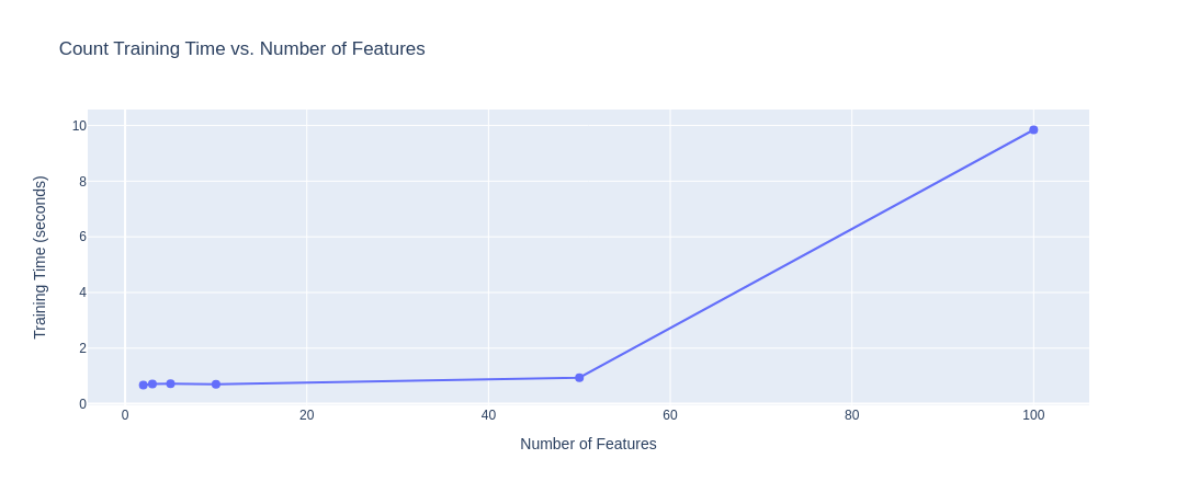
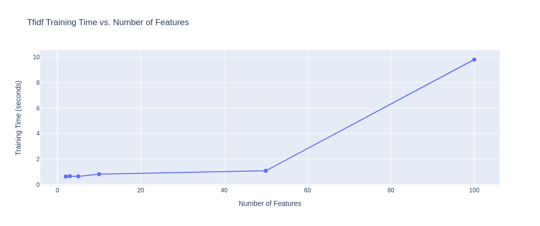
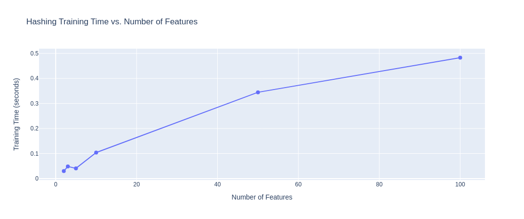
We first analyze the results obtained when attempting to fit a $K$-means model with $K=5$ (since we know we have five categories) for the various different embedding sizes: [2, 3, 5, 10, 50, 100]. To get these embedding sizes, we use LSA on the embeddings as described in the previous section. First, we plot the training times required for the various different embedding sizes to understand the computational overhead imposed by the increasing sizes:

Figure 14: Training Time vs. No. of Features (Count Vectorizer)

Figure 15: Training Time vs. No. of Features (TFIDF Vectorizer)

Figure 16: Training Time vs. No. of Features (Hashing Vectorizer)

Observation: From the above plots, we observe that up to an embedding size of $10$, for the count and TFIDF vectorizers, the training time is acceptable (within $2$ seconds), but once the embedding size is increased to $100$, the computational overhead grows $5x$. For the Hashing vectorizer, there is not a significant change (observe that the scale of the Y-axis is much smaller). Overall, these times are still very fast and reasonable for data preprocessing/analysis.

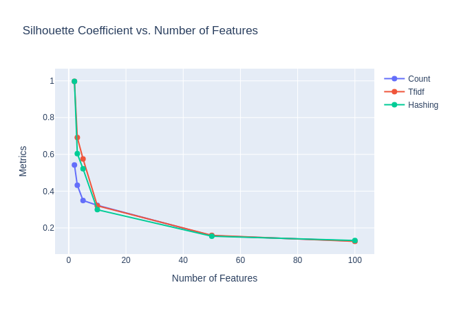
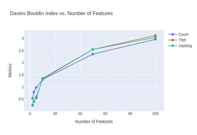
Next, we investigate some internal measures of the clustering to determine the intrinsic clustering quality:

Figure 17: Purity against No. of Features

Figure 18A: Silhouette coefficient against No. of Features

Figure 18B: Davies-Bouldin index against No. of Features

Observation: We observe from the purity plot that the ideal embedding size is around $10$, beyond this we do not see much increase in purity. This is further bolstered by the Silhouette coefficient and Davies-Bouldin index plots which illustrate that $10$ may be a point of reasonable tradeoff (elbow point) between true “clustering” structure and bad purity.

While the Silhouette coefficient and Davies-Bouldin index seem similar for the three embedding methods, the purity is highest for count vectoriser, followed by TFIDF and then the hashing vectoriser.

Before we proceed, we must further observe some external measures for our clustering. This is because, although the clustering may not be great for some of these embedding sizes, they may be more capable of capturing true (and more complicated) class structures. We plot below the plots for V-measure, which is identical to normalized mutual information (NMI):

Figure 19: NMI against No. of Features

Observation: The above plot further confirms our prior observation that the embedding of size $10$ might be the optimal embedding size for this task, as it performs the best when compared against the ground truth. The improvement for higher embedding sizes is negligible.

We also examine the same metrics for K-means using GloVe embeddings. Since the embedding dimensions are different, we do not combine the plots as the X-axis values are different, and the comparison of the metrics is more meaningful while controlling for embedding size.

Figure 20A: Results for K-Means with GloVe Embeddings (Davies Bouldin Score)

Figure 20B: Results for K-Means with GloVe Embeddings (Silhouette Score)

Figure 20C: Results for K-Means with GloVe Embeddings (Homogeneity Score)

Figure 20D: Results for K-Means with GloVe Embeddings (V-Score)

Observations:

• The Davies-Bouldin index plot shows that K-Means with GloVe embeddings are able to achieve scores between 0.64 and 0.74, far lower than the other methods before. This can be attributed to the fact that GloVe embeddings try to preserve linear sub-structure, and are trained on a large Twitter corpus where it learns good co-occurrence scores.
• The Silhouette Co-efficient shows that across all four dimension sizes, the K-Means models achieve scores around 0.63 and 0.64. This is a significant improvement as compared to other embeddings, and is likely attributed to the same reason as above.
• On the Homogeneity Score and the V-Measure, we see poor performance with GloVe embeddings. Our current hypothesis is that the low homogeneity score (and subsequently V-score) could be because the each article could contain competing themes of the various categories, though the category label only labels one dominant category. Since GloVe embeddings have a better estimation of the relationships of words (due to large pretraining), the model might be confusing these themes to label these articles in one or the other category. We seek to understand the cause of this more in future work.

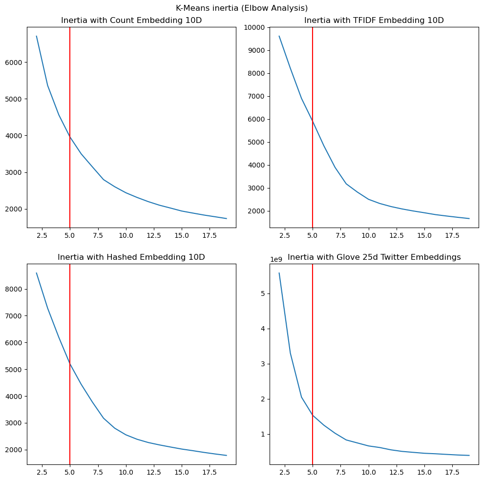
Categorisation of articles is an inherently ambiguous task with some additional sub categorisation possible. We expect that if the elbow is located somewhere in the vicinity of k=5, it will serve as a reasonable validation that our embeddings see some possible separation in the latent space.

We examine the change in the inertia (or sum of squared distances between cluster points and centroids) as we vary $k$ to see if this results in an “elbow” around k=5. Examining this using different embeddings could help us understand whether the different extracted/engineered features capture information that shows some grouping into topics. The figures have the ground truth category count $k=5$ marked as a red vertical line for readers’ reference.

Figure 21: Elbow Method for K-Means using inertia

Observation: We see that with GloVe embeddings there is a pronounced elbow around the area of $k=5$ and TF-IDF embeddings, we see a somewhat less pronounced elbow. With the other embeddings, it is possible that as they represent counts of individual terms, they continue to minimize the inertia with higher $k$, likely analogous to having more and more fine-grained topics.

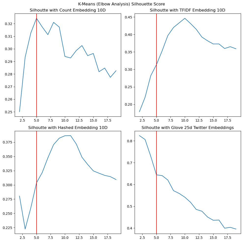
When we examine the Silhouette Score as we vary the number of clusters, we make a few observations as well. Figure 22 shows the variation of the Silhouette score variation with $k$.

Figure 22: Elbow Method for K-Means using Silhouette Score

Observation:

• With count embeddings, we see a peak in the Silhouette score around $k=5$ suggested good similarity within the points in a cluster, suggesting that count embeddings at 10 dimensions could give us some good clustering results.
• With TF-IDF and Hashed embeddings, we see a peak around 10 dimensions, which could be explained by the fact that the 10 principal dimensions are being modelled as distinct centres around that point.
• With GloVe embeddings, however, we notice that while the Silhouette score does not show a peak around $k=5$, it is significantly higher at 0.644, likely showing the ability of GloVe embeddings to create separable data due to its co-occurrence based training. In fact, we suspect that the reason the Silhouette score declines from $k=2$ could be because it is able to separate groups of categories cleanly at that point, while at higher scores, it contends with some overlap between these categories that is not captured in our labels as it is hard-clustering, while the real data might be more amenable to soft-clustering as in LDA.

Results Summary (scroll right to see the whole table):

Embedding	Homogeneity	Completeness	V-measure	Adjusted Rand-Index	Silhouette Coefficient	Fowlkes-Mallows Index	Calinski-Harabasz Index	Davies-Bouldin Index
Count Vector (10d)	0.43978	0.44316	0.44143	0.34189	0.31477	0.49231	5263.985	1.32094
Tf-IDF Vector (10d)	0.41463	0.42928	0.42171	0.39116	0.30749	0.53449	3867.35030	1.35666
Hashing Vector (10d)	0.28737	0.30519	0.29600	0.25811	0.29913	0.43699	4096.32769	1.32478
GloVe Vector (25d)	0.00535	0.01174	0.00735	-0.01008	0.64677	0.36697	22971.109584	0.64533

Hierarchical Agglomerative Clustering (HAC)

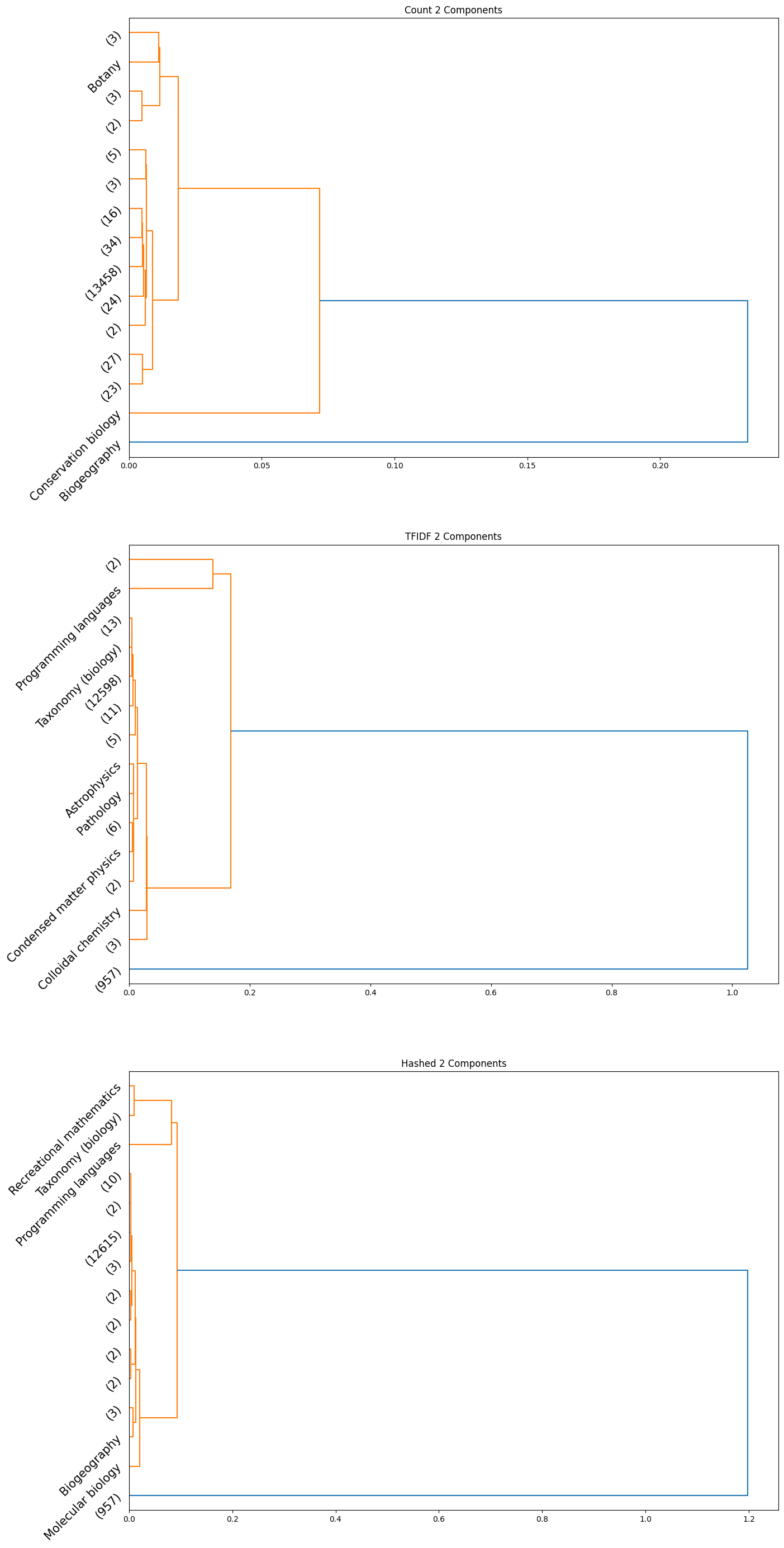
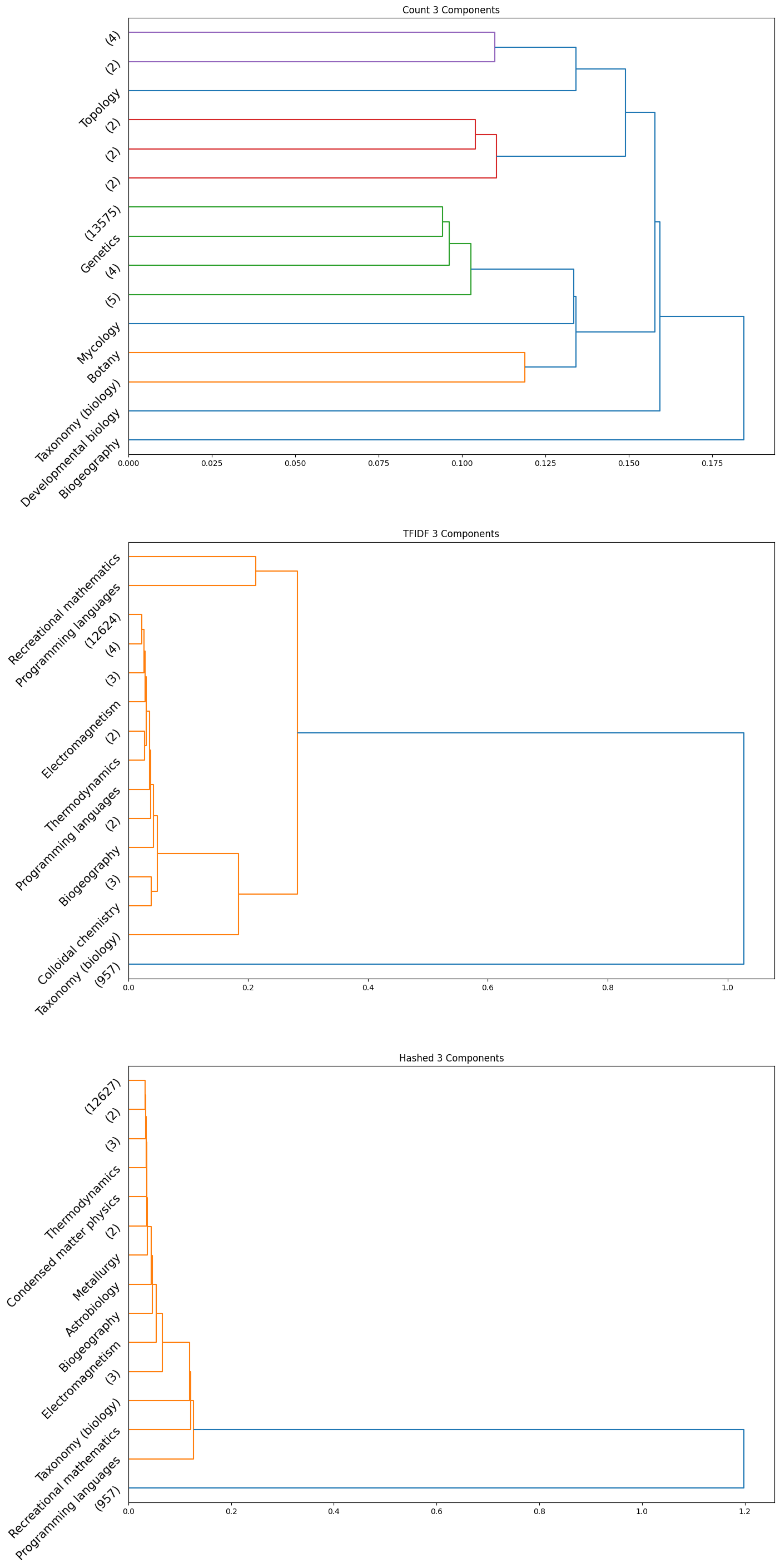
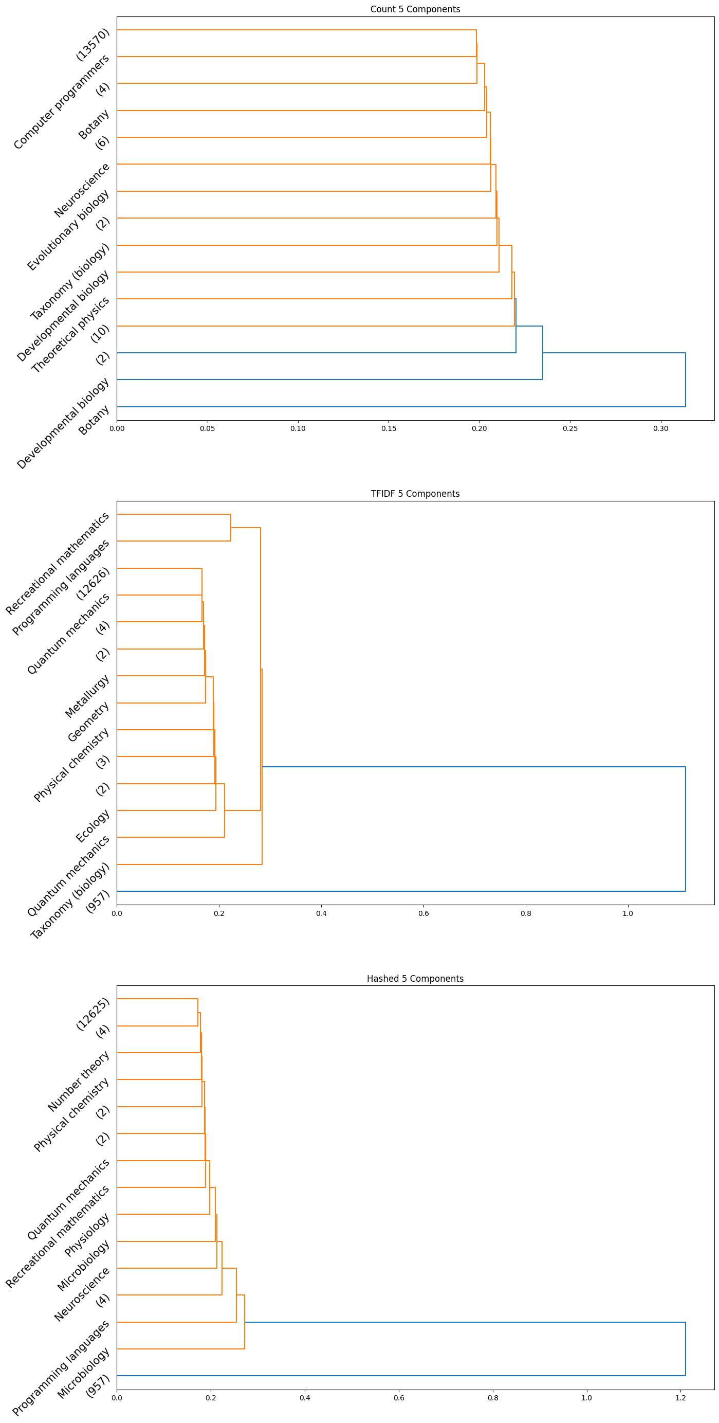
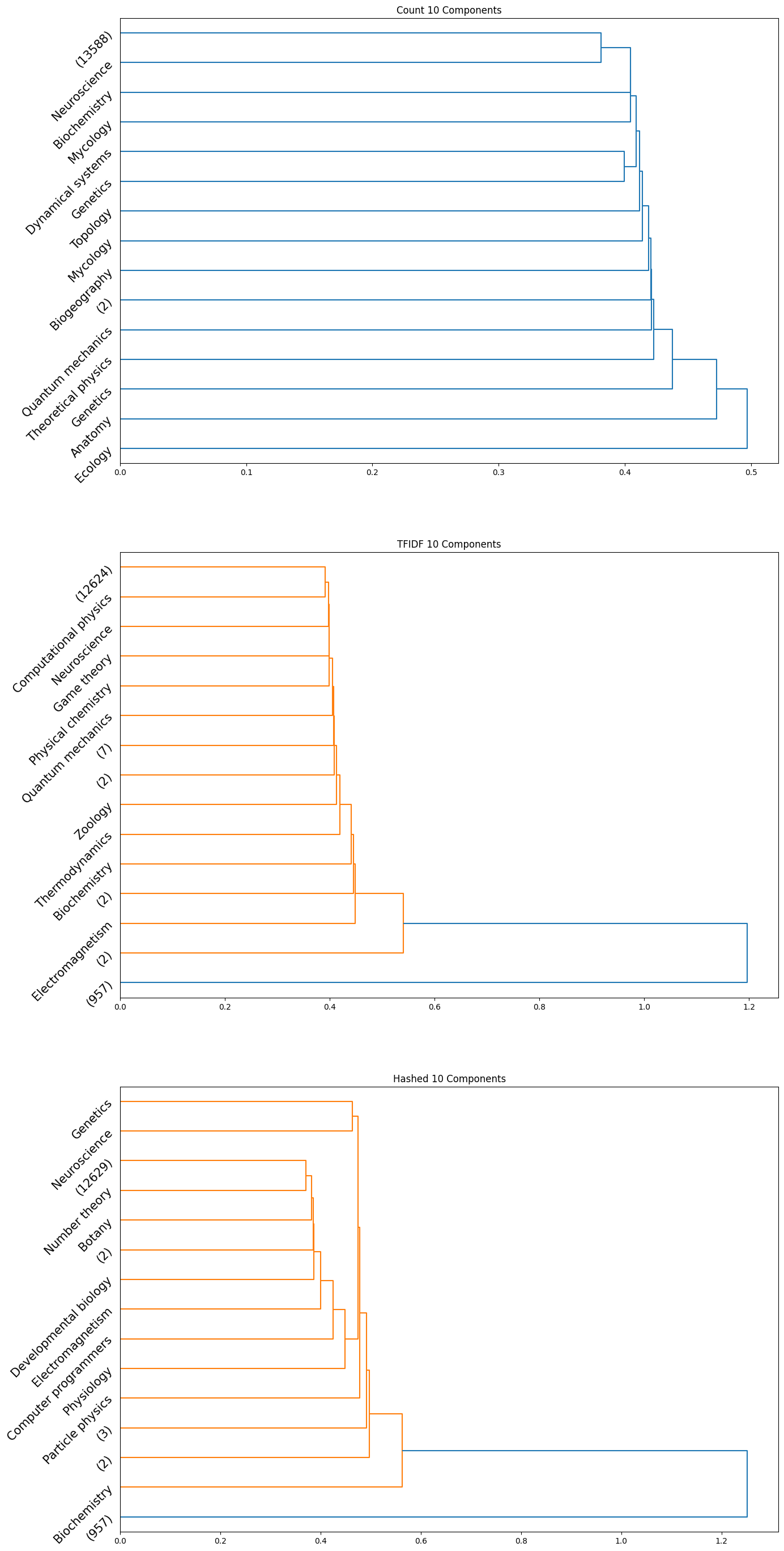
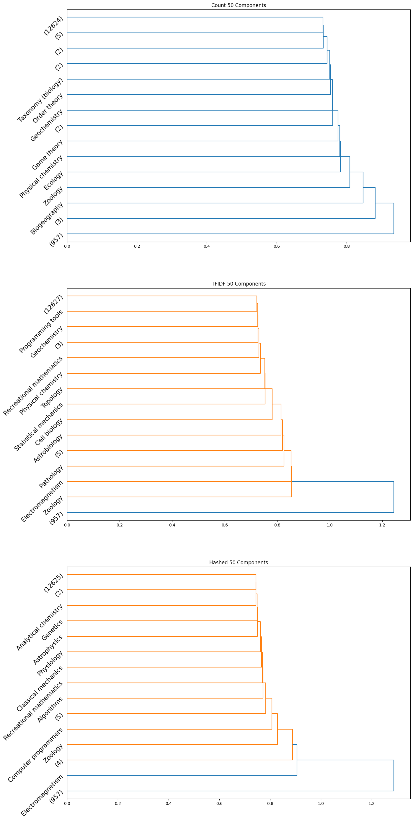
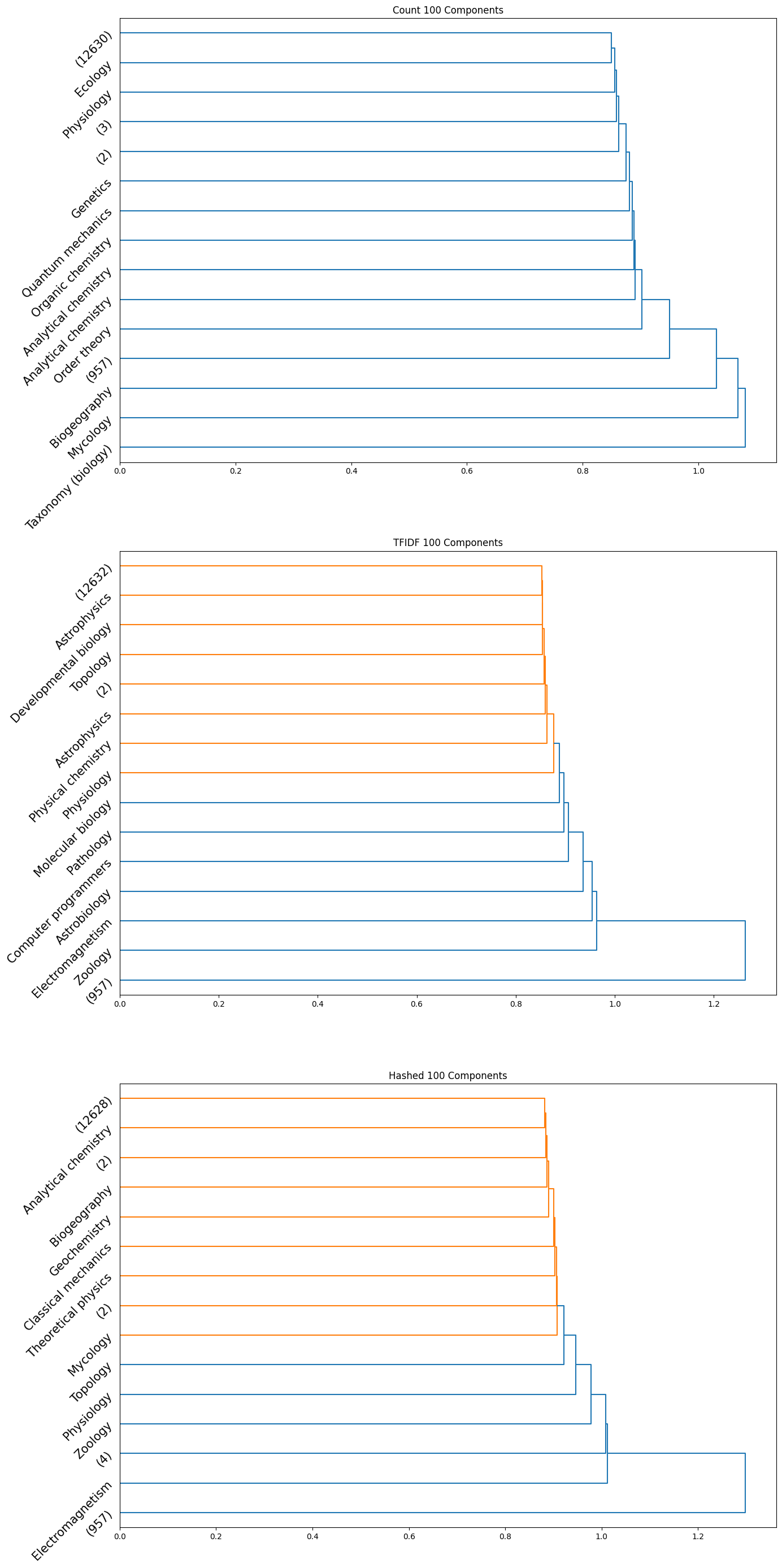
The accuracy results obtained for the HAC method were quite poor quantitatively; the maximum achieved adjusted rand index was only $0.006$. However, we did observe some insightful qualitative results. Interestingly, we can see from the plots obtained that the subcategories are frequently clubbed together under the HAC regime under the parent category. We used the ‘ward’ linkage criterion, which minimised the variance of the clusters that are merged. We provide below the plots of the dendrograms obtained for all cases for completeness:

Figure 23: Dendrogram for 2 component count, TFIDF, hashed

Figure 24: Dendrogram for 3 component count, TFIDF, hashed

Figure 25: Dendrogram for 5 component count, TFIDF, hashed

Figure 26: Dendrogram for 10 component count, TFIDF, hashed

Figure 27: Dendrogram for 50 component count, TFIDF, hashed

Figure 28: Dendrogram for 100 component count, TFIDF, hashed

Note that in the above plots, we have restricted to visualizing only the last $15$ clusters which were merged. Further, the class name is displayed only when the documents within a certain cluster only contain a single class; if not, the number of documents in the cluster is displayed in parentheses.

Observation: By observing the evolution of the dendrograms, we can make a few observations:

1. First and foremost, as we increase the sizes of the embedding, we are able to observe more and more “pure” clusters, i.e., clusters with just one class. This may be due to the fact that as the dimension size is increased, more information is available, i.e., more variance along newer directions are detected, and so the clustering occurs in a different order. Therefore, this allows for more precise clustering as the embedding size increases.
2. In general, all embeddings are able to often clump together subcategories of biology. This may however be due to the abundance of documents of the biology class as opposed to other classes.
3. The case of the count vectorizer with 3 components is particularly interesting since we see a truly nested structure in the dendrogram as compared to some of the other dendrograms where subcategories are incrementally segregated out. This case could therefore warrant further analysis.
4. Across all the number of candidate components, one can observe that the count vectorizer is much more prone to separating a single class into separate clusters. This can explained by the observation that a single sub-category does not necessarily have the same words repeated in a similar manner; it is likely a more sophisticated statistic, like the term frequency and document frequency combined that is suggestive of the sub category. By the same token however, it appears that count vectorizer is more strongly capable of clubbing together sub categories falling under a single parent category. Hence, there is a tradeoff at play here.
5. The TF-IDF and Hashed vectorizers seem to be generally more effective at isolating classes.
6. Finally, on an overall note, across all the embedding sizes and embedding methods, we can observe that biology gets grouped together rather effectively, but the model often wrongly clusters together some chemistry documents as well. This is not particularly surprising since there is a rather significant overlap between these two major fields. We can also observe that mathematics and physics subcategories often end up together, without a clear distinctive boundary between them. However, computer programming subcategories seem to subdivided only much further down in the dendrogram, as we don’t see much representation from such subcategories in the above plot.

Latent Dirichlet Allocation

We explore using LDA with stemming and without stemming, and qualitatively observe a better representation of topics with stemming. We also ensure to exclude some terms in the dataset which are not essential in order to boost the performance, such as “‘bibcode’, ‘doi’, ‘isbn’, ‘pmid’, ‘also’”. We find that the topics produced by LDA show a rough alignment with the categories in our dataset, with the representative terms helping us understand the mapping.

With stemming, we find the following topics, as in Figure 22.

Topic	Key Terms
Topic 1 (physics-like)	‘energi’, ‘quantum’, ‘particl’, ‘field’, ‘use’, ‘theori’, ‘system’, ‘equat’, ‘state’, ‘time’
Topic 2 (computer science-like)	‘use’, ‘function’, ‘theori’, ‘comput’, ‘system’, ‘number’, ‘set’, ‘one’, ‘retriev’, ‘quantum’
Topic 3	‘retriev’, ‘univers’, ‘scienc’, ‘theori’, ‘origin’, ‘research’, ‘archiv’, ‘natur’, ‘new’, ‘societi’
Topic 4 (chemistry-like)	‘chemic’, ‘use’, ‘reaction’, ‘acid’, ‘nuclear’, ‘cell’, ‘molecul’, ‘protein’, ‘electron’, ‘materi’
Topic 5 (biology-like)	‘water’, ‘cell’, ‘plant’, ‘soil’, ‘organ’, ‘dive’, ‘carbon’, ‘marin’, ‘ocean’, ‘use’

Observation: We see qualitatively that there is good alignment with the categories, with Topic 1 resembling Physics, Topic 4 resembling Chemistry, Topic 5 resembling Biology, Topic 2 resembling Computer Science and Topic 3 ambiguous, but still resembling either Physics or Chemistry. Since this approach allows documents to be represented by a combination of topics, it also hints to us that there are articles which are possibly a mix or topics, which is understandable since natural sciences usually relate to each other, and Computer Science and Mathematics overlap as well.

We also see reasonable results without stemming, but they are not as clear as the results above.

Supervised

Naive Bayes Classifier

We summarize the results obtained on training a Naive Bayes classifier on each of Count and TF-IDF vectorizers without dimensionality reduction, for category classification:

Count Vectorizer-based Naive Bayes
                        precision    recall  f1-score   support

   Branches of biology       0.90      0.88      0.89      1180
  Computer programming       0.93      0.91      0.92       462
 Fields of mathematics       0.83      0.90      0.86       562
Subfields of chemistry       0.79      0.73      0.76       590
  Subfields of physics       0.84      0.87      0.85       608

              accuracy                           0.86      3402
             macro avg       0.86      0.86      0.86      3402
          weighted avg       0.86      0.86      0.86      3402

TFIDF Vectorizer-based Naive Bayes
                        precision    recall  f1-score   support

   Branches of biology       0.60      0.97      0.74      1180
  Computer programming       1.00      0.59      0.74       462
 Fields of mathematics       0.85      0.74      0.79       562
Subfields of chemistry       0.94      0.31      0.47       590
  Subfields of physics       0.82      0.75      0.78       608

              accuracy                           0.73      3402
             macro avg       0.84      0.67      0.71      3402
          weighted avg       0.80      0.73      0.71      3402

Observation: From the above results, we observe that the count vectorizer performs exceedingly well, with an overall accuracy of $86$%. We can further verify that it is not simply overpredicting the majority class, by observing that reasonably high F1-scores are achieved across the various classes (with a minimum of only $76$% for “Subfields of chemistry”). We hypothesize that this is due to the count vectorizer’s ability to place emphasis on words that occur very frequently. Further, since the count vectorizer was already pruned during the embedding generation stage by removing those terms with document frequency greater than $25$%, it is effectively able to ignore unnecessary terms, and focus on meaningful terms. Also, notice that the macro average F1-score is also 86% which is a very good indication, since macro average prioritizes each class equally.

On the other hand, the TFIDF Vectorizer, while having a reasonable overall accuracy of $73$%, clearly faultier in the prediction of some classes. Interestingly, while it achieves a 100% precision on “Computer Programming”, it has a recall of $59$%, indicating that it is unable to prioritize words which are strongly linked to “Computer Programming” and will do so only for words very highly correlated with this class. A similar phenomenon is observed for “Subfields of Chemistry” with an unacceptably low recall of $31$%, i.e., Naive Bayes underpredicts for these 2 classes. Conversely, for “Branches of Biology”, it has a very high recall, with a relatively low precision of $60$%, i.e., it is overpredicting the class “Branches of Biology”. We hypothesize that this could be due to the fact the inverse document frequency too strongly prioritizes rarer terms, and so when a term which appears relatively rarely, but appears frequently in the category for “Branches of Biology”, Naive Bayes will be strongly biased toward selecting this class.

A point to note is that usually to maximise F1 score (especially on unbalanced data), we would need to tweak the binary threshold, but since we use one-vs-all classification here, we just choose the class which the highest probability.

We further attempted to make use of the dimension-reduced embeddings for the count and TFIDF vectorizer for Naive Bayes; however their performance were very suboptimal. This could be due to the fact that dimensionality reduction techniques like Latent Semantic Analysis (LSA) used here rely on PCA and SVD based methods, which do not (in general) eliminate conditional dependence. Hence, they do not result in any significant improvement in performance of the Naive Bayes classifier (in fact the performance becomes worse since two words in the lexicon which may have been conditionally independent in reality would potentially get eliminated since they are determined to share too much variance in the same direction). Regardless, we summarize here the best results obtained using Naive Bayes on the dimension reduced embeddings:

Results Summary:

Embedding	Accuracy (Micro F1)	Balanced Accuracy (Macro Recall)	Macro Precision	Macro F1-Score
Count Vector (10d)	0.39124	0.25849	0.42844	0.19617
Tf-IDF Vector (10d)	0.39095	0.25806	0.22842	0.19528

Random Forest Classifier

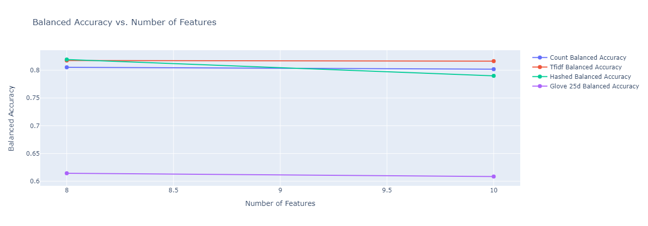
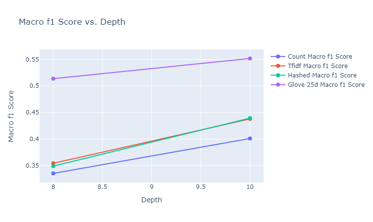
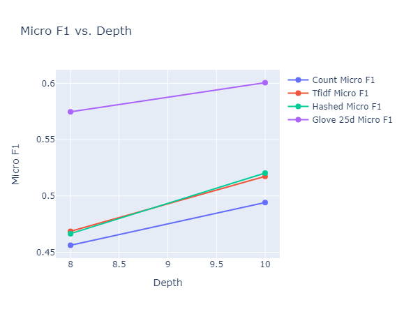
The final depths tested (after some hyperparameter running) for random forests were $8$ and $10$. We elucidate here the plots of our results for these depths to understand the tradeoff between computational complexity and model performance. We include here the plots for balanced accuracy, micro F1 and macro F1, which give an overall picture of classification performance, both with and without taking into account class imbalance.

Figure 29: Balanced Accuracy vs. Depth for Random Forest

Figure 30: Macro F1 vs. Depth for Random Forest

Figure 31: Micro F1 vs. Depth for Random Forest

Observations: We make the following observations:

1. Across almost all the metrics, we observe that increasing the depth from $8$ to $10$ results in either an improvement or no change in performance. This can be explained by the fact that affording a few more levels of branching for the random forest allows it to take more sophisticated decisions. One exception to this is the balanced accuracy of the hashed vectorizer, which takes a minor hit. This could be due to the fact that for the hashed vectorizer, it already reached the stage of overfitting.
2. While the GLoVe embeddings (for 25 dimensions) has a fairly low balanced accuracy, it has a significantly higher micro and macro F1 scores than any of the other embedding methods, achieving the highest test micro F1 score of 60% at a depth of $10$.

We provide the following raw result summary for perusal. Note that the count TFIDF, and hashed vectors here use the full components without dimensionality reduction, while the GLoVe vector is of 25 dimensions. We further report the results here for the depth of $10$ for the random forest, as it performs better. Finally, recall that for micro, precision is always the same as recall since the number of false positives and negatives would be the same. Hence it suffices to just keep track of the micro-F1, which is in fact the same as accuracy.

Results Summary:

Embedding	Accuracy (Micro F1)	Balanced Accuracy (Macro Recall)	Macro Precision	Macro F1-Score
Count Vector	0.49412	0.80186	0.38177	0.40083
Tf-IDF Vector	0.51734	0.81636	0.41155	0.43793
Hashing Vector	0.52028	0.78996	0.41585	0.43931
GloVe Vector	0.60053	0.60853	0.55693	0.55188

Gradient Boosting Classifier

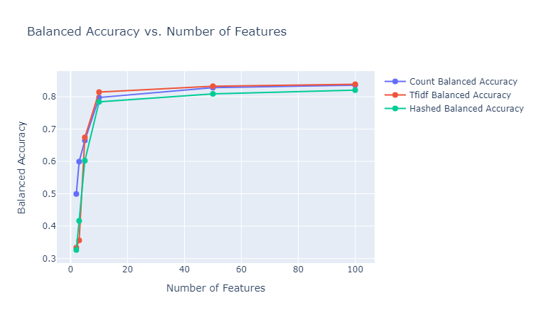
We make use of $50$ estimators with a learning rate of $1$ to test out the gradient boosting classifier (after some tuning). We provide here the plots of the performances of these classifiers for the various different embedding sizes, and state our observations. Note that the besides the results depicted below, we also tested using the GLoVe embedding of $25$ dimensions.

Figure 32: Balanced Accuracy vs. Number of Features for Gradient Boosting Classifier

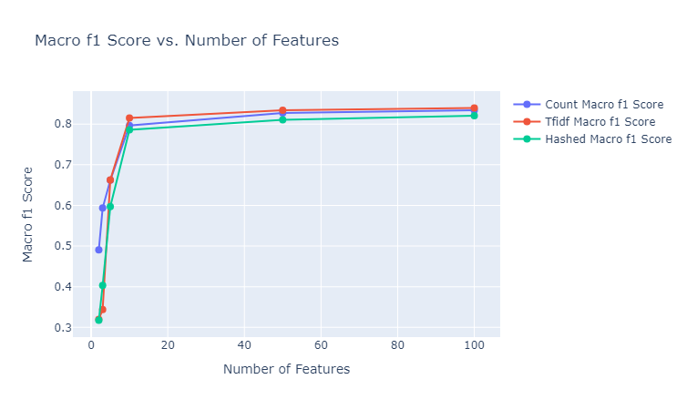Figure 33: Macro F1 vs. Number of Features for Gradient Boosting Classifier

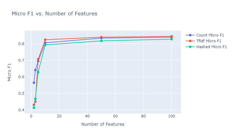Figure 34: Micro F1 vs. Number of Features for Gradient Boosting Classifier

Observations: We make the following observations:

1. We observe here a pattern similar to the performance pattern observed for a lot of the unsupervised clustering metrics, where the performance is quite high for the embeddings of size $10$, regardless of the embedding method, and then the increment in the metric is negligible.
2. The results here are significantly better than the random forest method, regardless of the embedding method. The best achieved micro F1 score here is $~85$% (TFIDF vectorizer of 100 dimensions) as opposed to $~60$% (glove 25d) for random forests. This aligns with the general expectation for the gradient boosting classifier as opposed to random forests, while however being more prone to overfitting.
3. The TFIDF vectorizer seems to consistently ourperform the other two vectorizers, as opposed to the superior performance of the count vectorizer for the Naive Bayes classifier. This can be explained by the fact that Naive Bayes classifier is a completely statistical method, mainly taking into account the counts of the various unique words across documents, and as a result the count vectorizer is a good fit for training such a model. On the other hand, gradient boosting makes use of decision trees to make sophisticated decisions, and finally applies boosting to provide corrections to the faults of the weak learners, and hence a more nuanced representation of the document which can encode importance of terms, like TFIDF, is capable of performing better.

Again, we provide here the raw results for some embeddings for perusal.

Results Summary:

Embedding	Accuracy (Micro F1)	Balanced Accuracy (Macro Recall)	Macro Precision	Macro F1-Score
Count Vector (10d)	0.80658	0.79777	0.79736	0.79653
TF-IDF Vector (10d)	0.825102	0.81450	0.81770	0.81513
Hashing Vector (10d)	0.79335	0.78437	0.78873	0.78580
GloVe Vector (25d)	0.83450	0.82831	0.82801	0.82740

Multi-Output Classifier

The Multi-Output Classifier handles joint classification tasks. Our current implementation of Multi-Output Classifier utilizes Random Forest as the estimator. To establish classification performance in tasks that have many classes, it’s important to compare against an appropriate baseline. Considering 143 subcategory classes, a classifier that outputs a random value would classify samples correctly $\frac{1}{143}$ of the time, if all classes had equal distribution.

Given that our subcategory classes are unbalanced, we calculate the random weighted baseline accuracy $acc_{rb}$ taking into account the proportion of samples of each class, expressed as:

\[acc_{rb} = \sum_{i=1}^{k}p_i^2\]

where $p_i$ is the proportion of samples with class $i$ in the training dataset. This gives us a random baseline accuracy of $1.38\%$. Similarly, we computed the baseline accuracy for category class to be $22.81\%$.

In both cases, model performance was much better than the baseline, subcategory classification reached close to 20%, and category classification reached 80%. The types of embedding did not affect the performance much. As expected, in the case of subcategory classification, given that we have 143 classes, the model needed more features to get to the optimal accuracy it can achieve.

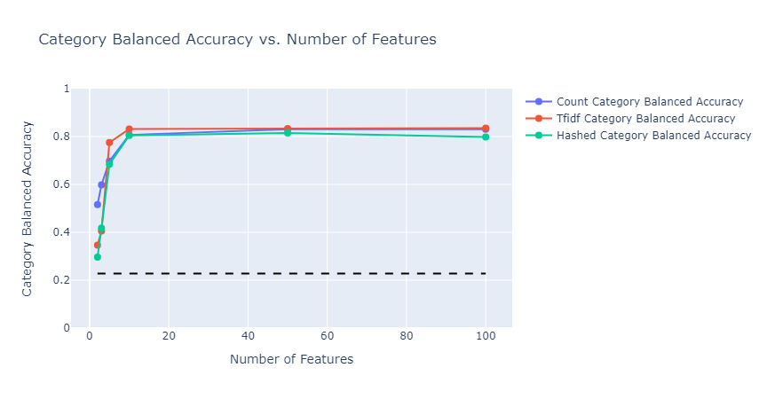Figure 35: Multioutput category classification Balanced Accuracy vs Number of Features

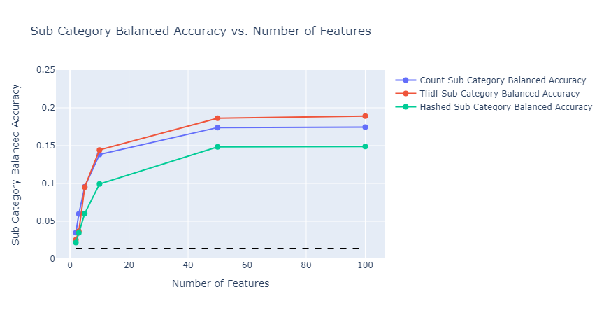Figure 36: Multioutput sub category classification Balanced Accuracy vs Number of Features

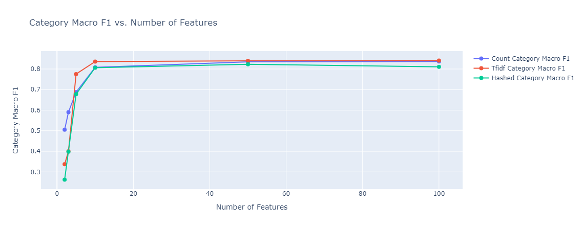Figure 37: Multioutput category classification Macro F1 vs Number of Features

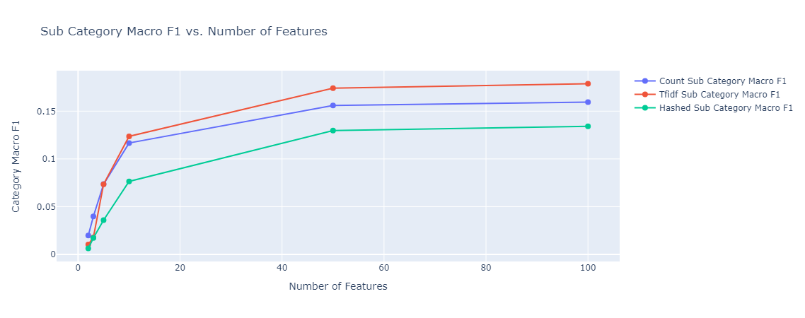Figure 38: Multioutput sub category classification Macro F1 vs Number of Features

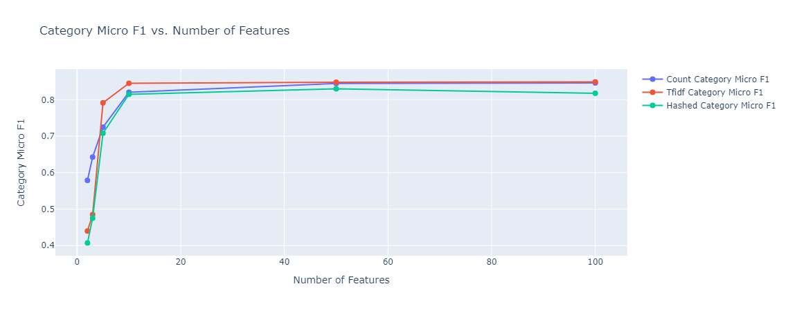Figure 39: Multioutput category classification Micro F1 vs Number of Features

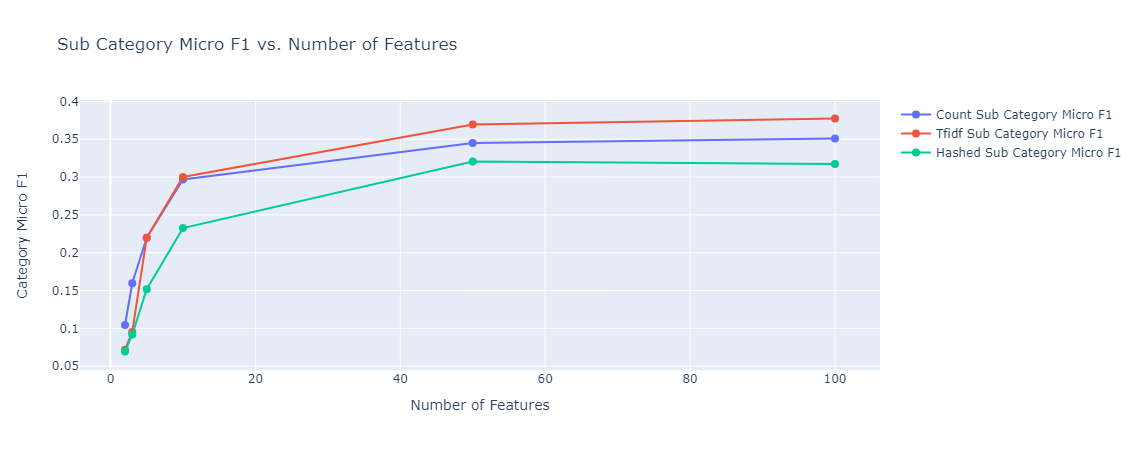Figure 40: Multioutput sub category classification Micro F1 vs Number of Features

Torchtext Embeddings

1. We try embedding dimensions of 64 and 128, and observe that embedding dimensions of 64 and 128 perform similarly, suggesting that sufficient information can be encoded in dimension 64 to do this classification. However if we intend to use that embedding for other tasks, we should consider testing on those tasks as well.
2. We plot confusion matrices on the validation set every epoch to see how it changes, and also on the test set to make observations on the types of errors.
   • We observe that the model quickly reduces errors and the heat map lights up on the leading diagonal, confirming good classification capability.
   • We don’t see heavy skew on any column despite seeing that the dataset is imbalanced towards one category. This confirms to us that the model is actually attempting to classify based on the representation and not always predict one class.
   • The change in the confusion matrix indicates what the model is learning. By epoch 1, we can already see that the model has learnt to classify the dominant classes (class 0, 4), but is making errors on the less prominent ones (1, 2,3). However thanks to our high learning rate and the schedule, we can see this quickly change, and by epoch 5, we see that classes 1,2,3 have been learnt as well.

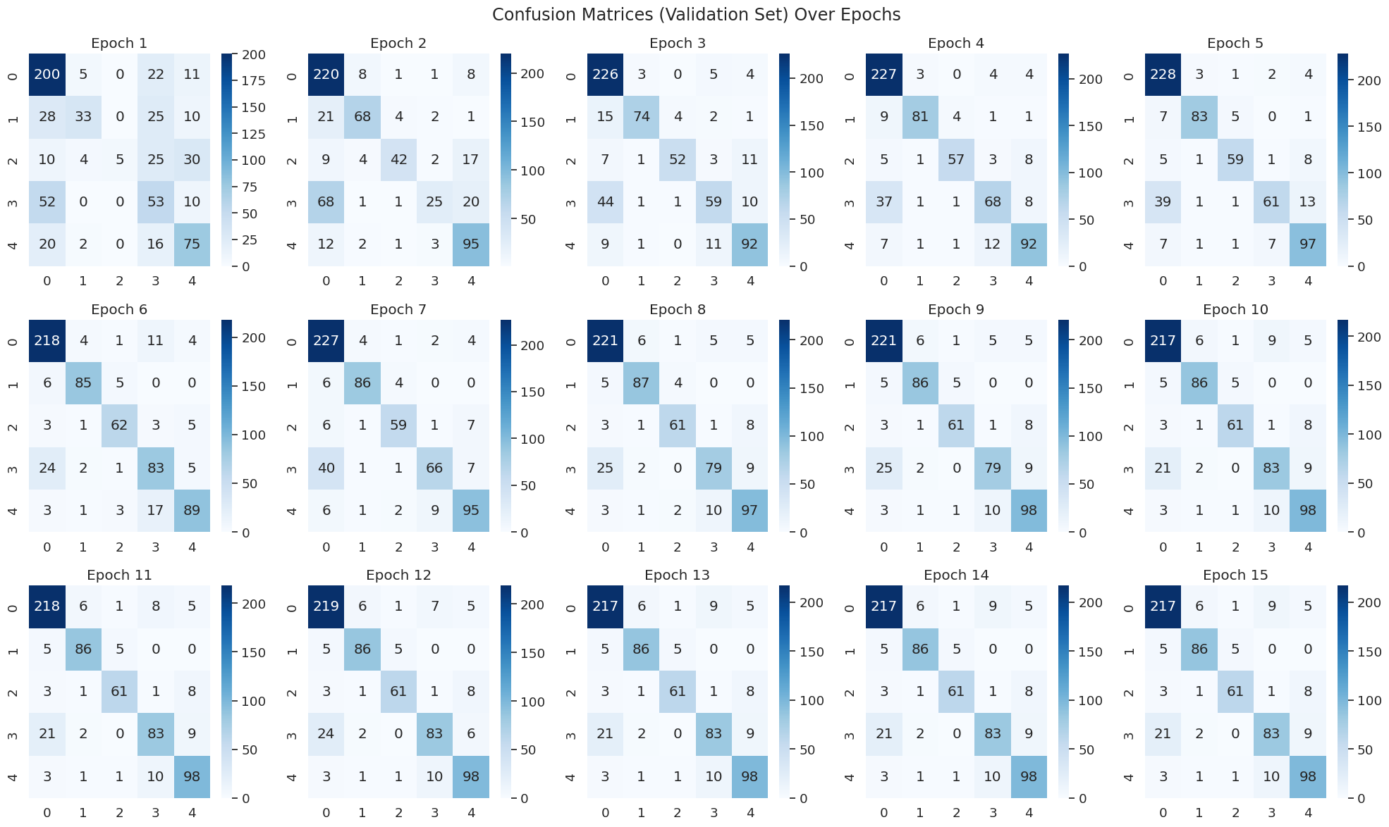Figure 40A: Confusion Matrix Changes During Training - Watching the model learn

1. The training and validation loss curves shows a steady and clean decline, and we can see that both plateau towards the end, showing convergence.

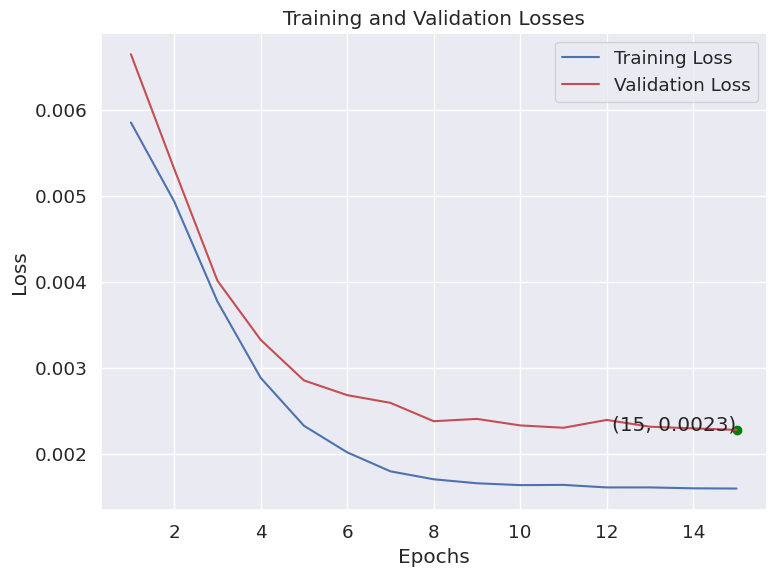Figure 40B: Training Characteristics - Training and Validation Loss show training stability

1. The learning rate decline matches the training loss curves. As the training loss declines below the validation loss, we see the scheduler quickly lower the learning rate to avoid overfitting or bouncing around. Without the scheduler, we would have likely seen large bounces in the loss as the optimizer jumped from one side to another.

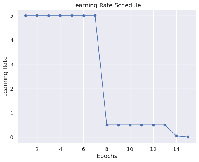Figure 40C: Benefiting from an adaptible learning rate - Step Learning Rate (initial = 5, gamma = 0.1)

1. The model is able to generalize well to the test set, achieving an overall accuracy = 85.6%. We further break down this result by exploring the confusion matrix as well as the precision and recall scores on individual categories.

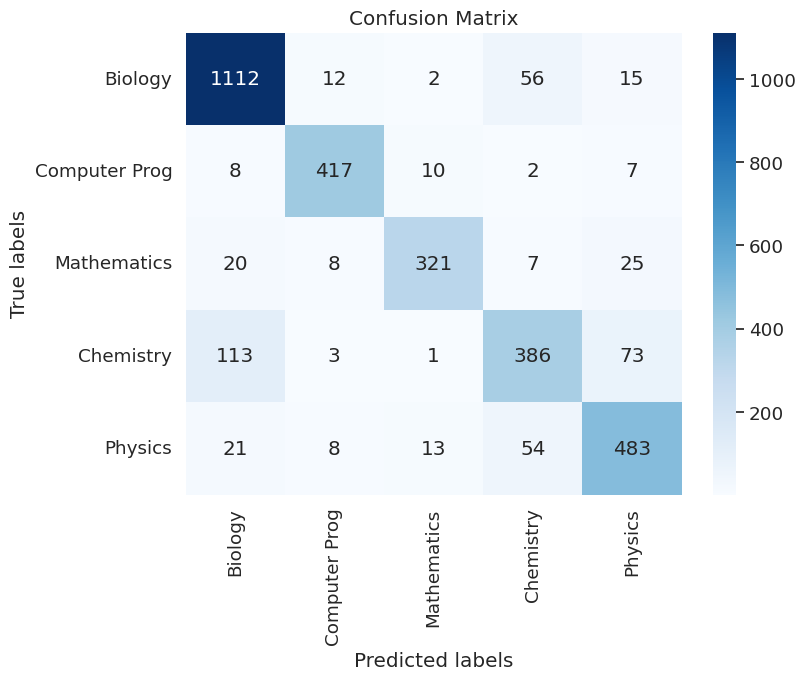Figure 40D: Confusion Matrix On Test Data - Testing the model’s generalizability

• Observation 1: The test confusion matrix shows that the leading diagonal (correct classification) is still dominant and confirms the accuracy score of 85.6%. This shows us that the learnt embeddings are useful enough to classify the text in these categories.
• Observation 2: The most common failure mode in the test set is that Chemistry pages are being confused for Biology. Since we can see that this common error mode is also the dominant error on the validation set during training, we hypothesize that the fields are similar and that the information provided in the dataset is likely insufficient to classify articles between these categories. It is also possible that in reality these pages might be interdisciplinary and be more amenable to soft clustering. Our work on topic modelling above supports this theory as well.
• Observation 3: Precision, Recall and Support Scores demonstrate consistent performance across classes, and confirms that the model is able to perform somewhat uniformly well across the test set. We observe that the recall score for Chemistry is particularly low, and this is explained by the confusion matrix showing that they are incorrectly labelled biology. We also see that the precision score for chemistry is lower than the rest at 76%. Once again, the confusion matrix confirms that this is because a number of Physics and Biology articles are incorrectly labelled as Chemistry, bringing down the precision score for the model.

             precision    recall  f1-score   support
  
    Biology       0.87      0.93      0.90      1197
  Computer Prog       0.93      0.94      0.93       444
    Mathematics       0.93      0.84      0.88       381
  Chemistry       0.76      0.67      0.71       576
    Physics       0.80      0.83      0.82       579
  
   accuracy                           0.86      3177
  macro avg       0.86      0.84      0.85      3177
   weighted avg       0.85      0.86      0.85      3177
  

Simple Linear Classifier

In order to draw meaningful conclusions about the quality of the embeddings we have, we also perform one final experiment by fitting ridge regression classifiers using cross-validation on the parentCategory classification task on the count and TF-IDF embeddings we extracted and also on polynomials of degrees 2 to 7 of the dataset. This analysis will help us understand whether we are limited by the quality of the representations we have, or the classification capacity of the models.

Experimental set up

We once again set up the classification task to classify the category using the embedded representations of the model obtained using TF-IDF and Count vectorizers. We perform ridge regression, and using cross-validation to select the alpha parameter. The main idea of using ridge classifier is to ensure that we don’t produce overfitting when working on polynomial degrees of the features. Since the glove embeddings explode in dimension when raised to a polynomial degree, we omit that from this experiment. We use RidgeClassifierCV out of the box from scikit-learn, and test in the range of alphas from [5e-4, 1e-3, 5e-2, 1e-2, 5e-1, 1e-1, 1].

Results

Ridge Classifier on TF-IDF and Count Vectors

The following are the accuracy scores obtained by RidgeClassifierCV on a test split of the dataset (15%).

Embedding	Accuracy Score
TF-IDF (10 dim)	81.5%
Count Vector (10 dim)	76.9%
Glove Twitter Embedding (25d)	43.3%

Observations:

• We clearly observe that the ridge classifier with TF-IDF and Count vectors show much better performance than the Glove embeddings despite being in lower dimensions. One possible reason for this is that the TF-IDF and Count scores directly identify words that are likely to be highly correlated with certain categories, whereas the Glove embeddings create more nuanced representations that capture the relative meanings between words. The RidgeClassifier may not have sufficient capacity to classify these.
• With just TF-IDF scores, we have already reached 81%, and we noted in the previous section that picking out our own embeddings did not go beyond 86% as well. This indicates that possibly we are limited in accuracy by the nature of the problem, where ambiguity regarding category has been resolved arbitrarily between classes that are close, and this might not be possible to capture without more training data.
• We also present the confusion matrices and classification score reports for each method below for reference.

TF-IDF:

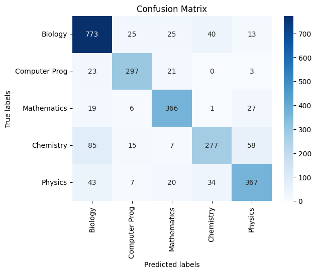*Figure 40E: Confusion Matrix On Test Data - Testing the model’s generalizability *

Classification Report:
               precision    recall  f1-score   support

      Biology       0.82      0.88      0.85       876
Computer Prog       0.85      0.86      0.86       344
  Mathematics       0.83      0.87      0.85       419
    Chemistry       0.79      0.63      0.70       442
      Physics       0.78      0.78      0.78       471

     accuracy                           0.82      2552
    macro avg       0.81      0.81      0.81      2552
 weighted avg       0.81      0.82      0.81      2552

Overall Accuracy: 0.8150

Count Vector:

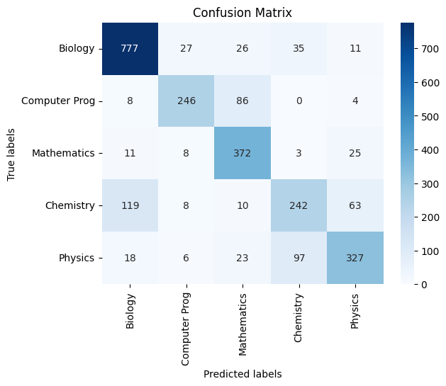*Figure 40F: Confusion Matrix On Test Data - Testing the model’s generalizability *

Classification Report:
               precision    recall  f1-score   support

      Biology       0.83      0.89      0.86       876
Computer Prog       0.83      0.72      0.77       344
  Mathematics       0.72      0.89      0.79       419
    Chemistry       0.64      0.55      0.59       442
      Physics       0.76      0.69      0.73       471

     accuracy                           0.77      2552
    macro avg       0.76      0.75      0.75      2552
 weighted avg       0.77      0.77      0.77      2552

Overall Accuracy: 0.7696

Glove Twitter 25d:

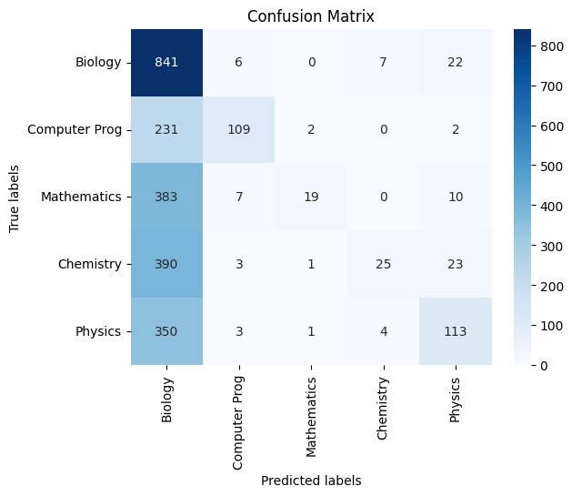*Figure 40G: Confusion Matrix On Test Data - Testing the model’s generalizability *

Classification Report:
               precision    recall  f1-score   support

      Biology       0.38      0.96      0.55       876
Computer Prog       0.85      0.32      0.46       344
  Mathematics       0.83      0.05      0.09       419
    Chemistry       0.69      0.06      0.10       442
      Physics       0.66      0.24      0.35       471

     accuracy                           0.43      2552
    macro avg       0.68      0.32      0.31      2552
 weighted avg       0.62      0.43      0.35      2552

Overall Accuracy: 0.4338

Ridge Classifier on Polynomial Features (TF-IDF and Count Vectors)

In this section, we perform polynomial transformations on the features and then assess the performance of the RidgeClassifierCV. The following table presents the results of this experiment.

Embedding Type	Polynomial Degree	Accuracy
Count Vector	1	76.96%
Count Vector	2	81.66%
Count Vector	3	83.31%
Count Vector	4	83.54%
Count Vector	5	83.89%
Count Vector	6	84.09%
TF-IDF Vector	1	81.50%
TF-IDF Vector	2	83.34%
TF-IDF Vector	3	84.16%
TF-IDF Vector	4	84.48%
TF-IDF Vector	5	84.44%
TF-IDF Vector	6	84.60%

Observations:

• We observe that the count vectorizer benefits significantly from adding 3 polynomial degrees and then the performance plateaus, possibly because the decision boundary ddoes not get more complicated than that.
• For the TF-IDF vectors, we see that polynomial transformations do not benefit the model significantly beyond a small performance improvement. It is possible that these representations separate the data linearly better than counts, resulting these results.
• These results also tell that we can achieve more than 80% on our classification task with these representations using just a simple classifier. Together with our previous experiment which creates its own embeddings, it hints that the limiting factor for our accuracy might be the fact that the data is inherently not cleanly separable and that many articles might actually be suitable for more than one category and arbitrarily labelled based on rules/human preference. As a result, we do not attempt training models with higher capacity to try and improve the performance.

We also produce confusions matrices and classification reports for these, but omit them in the interest of brevity.

Results Comparison

Now that we have tested several different supervised and unsupervised methods, we would like to compare and contrast the pros and cons of the different methods. Particularly, we aim to describe situations where some methods would be preferred over others.

First we summarize which models performed the best:

1. Among unsupervised methods, we note that the methods chosen serve different purposes and hence cannot be directly compared. However, from observation of K-means performance, we note that it would not be very effective for direct clustering of the subcategories as opposed to the hierarchical clustering. If we are only concerned with separating out clusters of documents into the 5 major branches, then K-means with TFIDF vectorizer gives reasonably good performance. Finally, the latest Dirichlet allocation (LDA) method allows us to generate important keyword terms identifying the different classes.
2. Among supervised methods, the best performing method was a simple linear classifier using our custom torchtext embeddings. The Naive Bayes classifier using the count vectorizer without dimension reduction had the next best performance. However, we would like to qualify this observation of “great performance” of the Naive Bayes classifier by highlighting that the Naive Bayes is highly dependent on the training dataset, and that this model works well within a specific dataset, but is likely not very useful for downstream tasks on other datasets. Then, we have the gradient boosting classifier using the TFIDF embeddings of $10$ dimensions (we ignore higher dimensions due to negligible increment in performance). Other embeddings for gradient boosting classifier also perform significantly well. However, after this, the performance falls off greatly for any of the other methods.

We systematically enlist the pros and cons of each method, and specify scenarios where each method may be useful:

1. Unsupervised
   • K-means: This method was fairly effective at separating out the $5$ parent categories into clusters.
     • Pros: This method scales well to larger datasets, and hence it can be straightforwardly applied to new domains as well, since we are able to generate clusters from the data which match the true categorization with better than random performances. So in the context of Wikipedia categorization, it can easily be directly applied to new pages that are added to Wikipedia.
     • Cons: It is highly sensitive to the specified number of clusters, which has to be chosen manually using either prior knowledge or analysis methods such as the elbow method. In our own analysis and elbow plots, we could notice directly this sensitivity to input parameters. So, while it can easily generalize to a new domain, in order to obtain satisfactory performance in the new domain, much manual tuning would still be needed.
   • Hierarchical Agglomerative Clustering (HAC): The purpose of this method is to obtain a hierarchy of clusters.
     • Pros: This method is effective at isolating parent and subcategories successively, compared to the K-means method as evidenced by the dendrogram plots analyzed earlier. It is therefore very useful in the context of analyzing the distribution of a particular spatial representation of the text data.
     • Cons: This method is (relatively) computationally intensive, and the visualizations and insights that can be derived become meaningless once the data becomes too large. In fact, when we applied this method for our task, a large amount of fine-tuning for our visualization had to be done in order to derive insights from it; when applying this to a newer dataset with much larger number of data points, it may be an infeasible route to derive insights. Cutting off the implied dendrogram can also be a relatively arbitrary choice that requires much manual tuning.
   • Latent Dirichlet Allocation (LDA): The purpose of this method was to explore the data qualitatively and understand whether there were any characteristics that made certain classes inherently confusion. By extracting 5 prominent topics from this dataset using the topic model, and examining their key words, we were able to see that there are strongly shared themes between the classes the models tended to often mis-classify (such as Biology and Chemistry). It also gave us a qualitative view of the themes in the dataset.
     • Pros: It produced human interpretable topics that gave an intuitive sense of the dataset, and it runs quickly and in an unsupervised fashion
     • Cons: The approached is limited by its inability to use our pre-trained embeddings, and works on co-occurences of words across documents. While a useful exploratory tool, it was not beneficial to our classification task directly.
2. Supervised
   • Naive Bayes: This extremely simple method is effective at making predictions for the parent categories.
     • Pros: This method is extremely efficient as it is a purely probabilistic method. In fact, this is one of the major reasons why the count vectorizer works exceedingly well for Naive Bayes as opposed to other supervised methods; there is quite a strong correlation between the counts of certain keywords and the true category. Further, this method can directly applied to other domains where the distribution of terms would be roughly similar.
     • Cons: This is an overly simplistic method, since it makes the assumption of conditional independence among the features. In reality, this is likely not true; sequences of words are sometimes more important patterns than individual words but Naive Bayes would assume that each word in the sequence would be independent from the other. Hence, Naive Bayes can be quite bad at disambiguation. For instance, “quantum” is a term that appears both in the topic of quantum physics as well as CPU scheduling. But Naive Bayes would be unable to distinguish between these $2$ contexts directly. A smarter model may look for the phrase “time quantum” to correlate with CPU scheduling, as opposed to “quantum tunnel” (for instance) to correlate with quantum physics. Other models like random forests, and the decision-tree based gradient boosting make decisions based (hopefully) on sequences of words, and hence have a greater change of disambiguating more effectively.
   • Random Forest Classifier: This method utilizes the technique of bootstrap aggregating (bagging) and is also fairly effective at predicting the parent categories.
     • Pros: Random forests are implicitly capable of performing feature selection, since they find the features to split on by construction. This allows us to make use of the entire feature space directly without dimensionality reduction, hence eliminating the intermediate step of determining the optimal reduced dimension for representation. Further, since it averages across a set of weak learners to create one strong learner with reduced variance thus reducing the chance of overfitting.
     • Cons: Even for our relatively small dataset, the random forest was computationally intensive, taking a significant amount of time to train. If our models here were to be adapted to an online setting, so that it could keep retraining based on new data, the computational cost would be heavy. Also, these models are not very directly interpretable since they achieve better performance by training weak learners on varying distributions of the same training data. Hence, without direct access to and detailed analysis of these instantiations of distributions, interpretability cannot be derived from the random forest model.
   • Gradient Boosting Classifier: This method utilizes the technique of boosting, and shows greater effectiveness at predicting the parent categories than the random forest classifier.
     • Pros: It is able to significantly outperform the random forest classifier as we highlighted earlier. This is due to the fact that unlike random forests, the gradient boosting classifier uses the principle of boosting which targets the samples on which previous weak learners make errors. As a result, its generalization capability is better. So it can effectively classify new Wikipedia articles.
     • Cons: Due to the very design choice that allows gradient boosting to outperform random forests, its computation cannot be parallelized; it must have information from the previous weak learner (decision tree), in order to train the next weak learner. As a result, it has a significant computational cost, which we also observed in our relatively small dataset. Furthermore, gradient boosting is very susceptible to noise in the training data, and hence may overfit much more than the random forest. Although we do not observe such a significant difference in our experiments, this may become a very significant factor when applied to a larger set of interrelated/similar topics.
   • Multi-Output Classifier:
     • Pros: This has an extended capablity of predicting both category and subcategory variables. It is capable of capturing correlation beween categories and subcategories and hence shows improved balanced accuracy score over training models individually for category and subcategory target variables. Since category and subcategory values are correlated it is better to build a single model capable of predicting both these values as it also requires lower training time and results in a better accuracy. For example, employing a count vectorizer with 10 features and a random forest depth of 10 resulted in a balanced accuracy of 80.18%, whereas utilizing multi-output for category predictions achieved a higher balanced accuracy of 82.15%. Through exploratory data analysis, we determined the baseline accuracy for the distribution of category to be 0.2281 and subcategory to be 0.0138. Figures 35 and 36 illustrate the balanced accuracy for both categories and subcategories are much better than the baseline indicating the multioutput performed well.
     • Cons: When dealing with multiple outputs, the model’s susceptibility to noise or irrelevant features might be amplified, potentially affecting the overall performance, especially in cases where outputs are interrelated or influenced by similar factors. The model failed to capture the correlation between category and subcategory in some cases resulting in misclassifications. The analysis results were recorded as follows: 1830 instances where the model correctly predicted only the category, 69 instances where it correctly predicted only the subcategory, 1002 instances where it accurately predicted both the category and subcategory simultaneously, and 501 instances where it did not correctly predict either.
   • Learned Embeddings and Linear Classifier: In this method, we learned embeddings for words by trying to use the loss from the classification function as a gradient direction. The model used a bag of words approach to generate the emebddings for texts, and then used this for classification.
     • Pros: Simple and quick approach that does not rely on pre-trained embeddings. It also yields an embedding matrix that can be used for other tasks.
     • Cons: The limiting assumption here is the bag of words model and the lack of non-linearity in the linear classifier after it. These prevent the model from generalizing to complex boundaries, but enable us to see the separability of the embeddings and understand their value better when we use a linear probe.

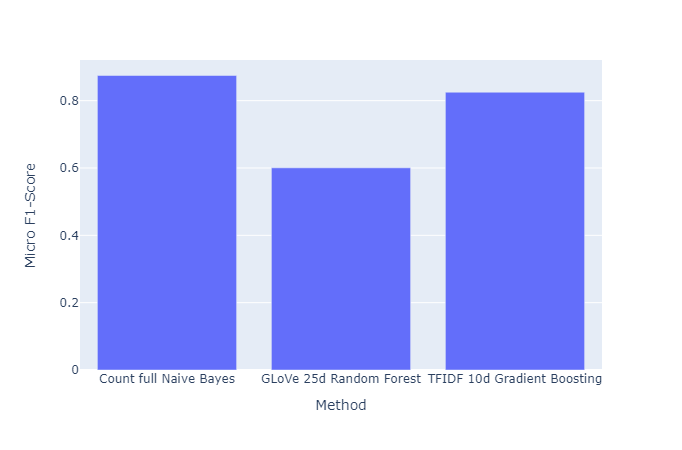
We provide below summary plots of the best performing supervised methods for quick comparison:

Figure 41: Balanced Accuracy vs. Method

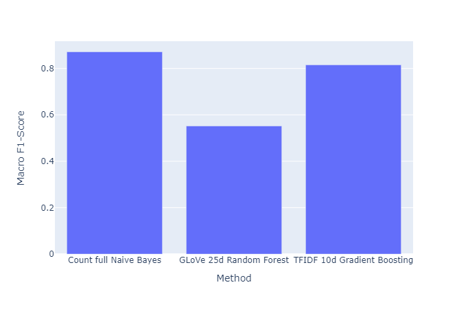Figure 42: Macro F1 vs. Method

Figure 43: Micro F1 vs. Method

Conclusion

At this juncture, we would like to summarize the main findings of our analysis, and explain how our work can find applications for Wikipedia categorization.

In short, in this project, we tested and analyzed several supervised and unsupservised machine learning method for the categorization of Wikipedia into $5$ major categories. To do this, we retrieved several Wikipedia articles by the $5$ major categories we chose, along with their subcategories as well. Then, we first performed some exploratory analysis to understand our data better. One of the major insights was the relatively uneven spread of documents we retrieved, with the class “Branches of Biology” dominating the other classes.

We then create word embeddings from our documents to express them in some latent space, so that they can be applied for machine learning algorithms. For this we choose to use $3$ standard methods of Count, TFIDF, and Hashed vectorizers. Further, we note that the embeddings generated via these methods have a very large dimension, and hence make use of Latent Semantic Analysis (LSA) to reduce the dimensionality of our latent space. We store several candidate reduced dimension latent space representations, to determine which can perform the best. Then we also use Twitter’s GLoVe embeddings, for a more sophisticated deep learning based word embedding, and also maintain different latent spaces for these using LSA.

For unsupervised techniques, we make use of K-means, which we observed yields reasonable performance for segregating the $5$ major clusters, especially with the TFIDF embedding of 10 dimensions. Then, we attempted to the hierarchical agglomerative clustering method, which, while giving bad overall performance, lent some very good insights into the clustering of our data in the latent space. Finally, Latent Dirichlet Allocation (LDA) gives us a highly interpretable result of the terms based on which the greatest distinction between classes can be found, and highlighted some possible reasons for the difficulties faced by our clustering models.

For supervised techniques, we first attempt the simplistic Naive Bayes classifier, and observe the best performance with the Count Vectorizer (without dimensionality reduction) for this specific dataset. However, we qualify this statement by highlighting the high dependence of Naive Bayes on the training dataset, and move on to attempt other supervised methods. We next attempt random forests, to determine the performance of bagging for our dataset. We observe sub-optimal performance, but note the dependence of the performance on the depth allowable for the random forests. Finally, we make use of gradient boosting classifier, which yields the best performance (apart from Naive Bayes) with the 25-dimensional GLoVe embeddings.

Overall, we believe that the gradient boosting classifier provided the best performance, and would be the best choice for a downstream classification task. However, we also note here that the choice of the “best classifier” is highly task-dependent, and the best option would always likely be a combination of the methods tested in this report.

Limitations and Future Improvements

We would now like to highlight the limitations of our work, and future directions to continue this work. Firstly, we only consider $5$ major categories; Wikipedia articles have a wide range of categories of articles, which we do not touch upon in our project. Further, our methods are heavily dependent on knowing these categories a priori for the purpose of prediction; a more sophisticated method would be topic modelling which should, ideally, be able to extract the topic for a certain document in an unsupervised manner without labels. To help guide future work in this direction, we briefly explored topic modelling through LDA, to show that this is feasible.

Also, currently, our work does not take into consideration documents of other languages (an area Wikimedia Foundation themselves worked on), which would require further effort to develop language-specific embeddings in order to correctly capture context.

Integrating ML into a production system is also a challenging task, and is required for this to be useful in the real world. Based on these limitations, we propose the following future avenues for improvements:

1. The model can be transformed to a pipeline that constantly scrapes Wikipedia category data and relevant documents.
2. A combination of supervised and unsupervised topic modelling predictions can be used to either generate an existing category for the article, or to generate a new category for the article on-the-fly.
3. Wikipedia articles of different languages can be dealt with separately, and language-specific embeddings can be made use of to similarly automatically generate categories.
4. Online learning approaches can be explored to avoid re-training on the very large Wikipedia dataset repeatedly
5. An additional UNKNOWN category can be predicted for articles that don’t fit into any existing category. This can highlight articles that need human attention for creation of a new category.

---

Team Member Contribution Table (Final Report)

Name	Contribution
Siddharth M. Sundaram	Hierarchical Agglomerative Clustering (HAC); Random Forest; Gradient Boosting; Naive Bayes; Report Writeup
Sashankh C. Kumar	Embedding Training and Linear Probe; Ridge Classifier; Result Comparison; Report Writeup
Mathan Mahendran	Data cleaning pipeline; Dataset/LSA Visualisation; Report Writeup; Presentation Slides
Preethi N. Murthy	Data cleaning pipeline; Dataset/K-means Visualisation; MultiOutput Classifier; Report Writeup; Slides and Video
Siddharth Sriraman	Results Analysis (multi-output classifier, supervised models); Report Writeup; Slides and Video

---

Team Member Contribution Table (Midterm Report)

Name	Contribution
Siddharth M. Sundaram	Embeddings Generation (CountVec, HashingVec, Tf-Idf); LSA; K-means; Report Writeup
Sashankh C. Kumar	Embeddings Generation (GloVe); LDA; LSA; K-means (Elbow Method); Report Writeup
Mathan Mahendran	Data cleaning pipeline; Dataset/LSA Visualisation;
Preethi N. Murthy	Data cleaning pipeline; Dataset/K-means Visualisation;
Siddharth Sriraman	Data cleaning pipeline; Dataset/LSA Visualisation; Report Writeup

---

Team Member Contribution Table (Proposal)

Name	Contribution
Siddharth M. Sundaram	Proposal Writeup; Dataset Collection
Sashankh C. Kumar	Video; Presentation Slides;
Mathan Mahendran	Gantt Chart; Proposal Writeup
Preethi N. Murthy	Video; Presentation Slides
Siddharth Sriraman	Video; Presentation Slides

---

---

Project Timeline

---

---

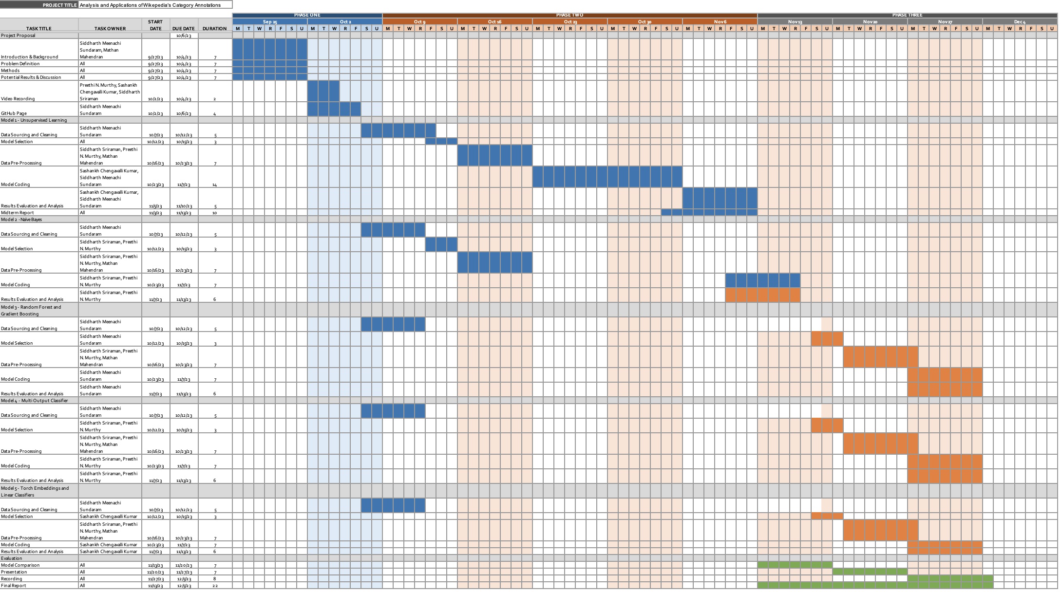
Video link: CS7641 Group 41 Proposal

---

References

[1] I. Johnson, M. Gerlach, and D. Sáez-Trumper, “Language-agnostic topic classification for Wikipedia,” arXiv.org, https://arxiv.org/abs/2103.00068v1 (accessed Oct. 1, 2023).

[2] Nastase, Vivi & Strube, Michael. (2008). “Decoding Wikipedia Categories for Knowledge Acquisition.” Proceedings of the National Conference on Artificial Intelligence. 2. 1219-1224.

[3] M. Allahyari and K. Kochut, “Semantic Tagging Using Topic Models Exploiting Wikipedia Category Network,” 2016 IEEE Tenth International Conference on Semantic Computing (ICSC), Laguna Hills, CA, USA, 2016, pp. 63-70, doi: 10.1109/ICSC.2016.34.

[4] Z. Syed, T. Finin, and A. Joshi, “Wikipedia as an Ontology for Describing Documents”, ICWSM, vol. 2, no. 1, pp. 136-144, Sep. 2021.

[5] Jeffrey Pennington, Richard Socher, and Christopher D. Manning. 2014. “GloVe: Global Vectors for Word Representation.”